A Tale of Three Cosines—An Experimental Mathematics Adventure
Identifying Peaks in Distributions of Zeros and Extrema of Almost-Periodic Functions: Inspired by Answering a MathOverflow Question
One of the Holy Grails of mathematics is the Riemann zeta function, especially its zeros. One representation of ![]() is the infinite sum
is the infinite sum ![]() . In the last few years, the interest in partial sums of such infinite sums and their zeros has grown. A single cosine or sine function is periodic, and the distribution of its zeros is straightforward to describe. A sum of two cosine functions can be written as a product of two cosines,
. In the last few years, the interest in partial sums of such infinite sums and their zeros has grown. A single cosine or sine function is periodic, and the distribution of its zeros is straightforward to describe. A sum of two cosine functions can be written as a product of two cosines, ![]() . Similarly, a sum of two sine functions can be written as a product of
. Similarly, a sum of two sine functions can be written as a product of  . This reduces the zero-finding of a sum of two cosines or sines to the case of a single one. A sum of three cosine or sine functions,
 ![]() , is already much more interesting.
, is already much more interesting.
Fifteen years ago, in the notes to chapter 4 of Stephen Wolfram’s A New Kind of Science, a log plot of the distribution of the zero distances…

… of the zero distribution of ![]() —showing characteristic peaks—was shown.
—showing characteristic peaks—was shown.
And a recent question on MathOverflow.net asked for the closed forms of the positions of the maxima of the distribution of the distances of successive zeros of almost-periodic functions of the form ![]() for incommensurate
for incommensurate ![]() and
and ![]() . The post showed some interesting-looking graphics, the first of which was the following (
. The post showed some interesting-looking graphics, the first of which was the following (![]() is the golden ratio) for the distance between successive zeros (taking into account the first 100k positive zeros):
is the golden ratio) for the distance between successive zeros (taking into account the first 100k positive zeros):

At first, one might be skeptical seeing such an unusual-looking histogram, but a quick one-liner that calculates all zeros in the intervals ![]() and
and ![]() does confirm a distribution of the shape shown above as a universal shape independent of the argument range for large enough intervals.
does confirm a distribution of the shape shown above as a universal shape independent of the argument range for large enough intervals.
 ✕
Function[x0, Histogram[Differences[
     t /. Solve[
      Cos[t] + Cos[GoldenRatio t] + Cos[GoldenRatio^2 t] == 0 \[And]
       x0 < t < x0 + 10^3 \[Pi], t]], 200]] /@ {0, 10^6}
|

And the MathOverflow post goes on to conjecture that the continued fraction expansions of ![]() are involved in the closed-form expressions for the position of the clearly visible peaks around zero distance
are involved in the closed-form expressions for the position of the clearly visible peaks around zero distance ![]() , with
, with ![]() 1, 1.5, 1.8 and 3.0. In the following, we will reproduce this plot, as well as generate, interpret and analyze many related ones; we will also try to come to an intuitive as well as algebraic understanding of why the distribution looks so.
1, 1.5, 1.8 and 3.0. In the following, we will reproduce this plot, as well as generate, interpret and analyze many related ones; we will also try to come to an intuitive as well as algebraic understanding of why the distribution looks so.
It turns out the answer is simpler, and one does not need the continued fraction expansion of ![]() . Analyzing hundreds of thousands of zeros, plotting the curves around zeros and extrema and identifying envelope curves lets one conjecture that the positions of the four dominant singularities are twice the smallest roots of the four equations.
. Analyzing hundreds of thousands of zeros, plotting the curves around zeros and extrema and identifying envelope curves lets one conjecture that the positions of the four dominant singularities are twice the smallest roots of the four equations.

Or in short form: ![]() .
.
The idea that the concrete Diophantine properties of ![]() and
and ![]() determine the positions of the zeros and their distances seems quite natural. A well-known example where the continued fraction expansion does matter is the difference set of the sets of numbers
determine the positions of the zeros and their distances seems quite natural. A well-known example where the continued fraction expansion does matter is the difference set of the sets of numbers ![]() for a fixed irrational
for a fixed irrational ![]() (Bleher, 1990). Truncating the set of
(Bleher, 1990). Truncating the set of ![]() for
for ![]() , one obtains the following distributions for the spacings between neighboring values of
, one obtains the following distributions for the spacings between neighboring values of ![]() . The distributions are visibly different and do depend on the continued fraction properties of
. The distributions are visibly different and do depend on the continued fraction properties of ![]() .
.
 ✕
sumSpacings[\[Alpha]_, n_] :=
 With[{k = Ceiling[Sqrt[n/\[Alpha]]]}, Take[#, UpTo[n]] &@N@
    Differences[
     Sort[Flatten[
       Table[N[i + \[Alpha] j, 10], {i, Ceiling[\[Alpha] k]}, {j,
         k}]]]]]
|
 ✕
ListLogLogPlot[Tally[sumSpacings[1/#, 100000]],
                              Filling -> Axis,
   PlotRange -> {{10^-3, 1}, All},
   PlotLabel -> HoldForm[\[Alpha] == 1/#],

   Ticks -> {{ 0.01, 0.1, 0.5}, Automatic}] & /@ {GoldenRatio, Pi,
  CubeRoot[3]}
|

Because for incommensurate values of ![]() and
and ![]() , one could intuitively assume that all possible relative phases between the three cos terms occur with increasing
, one could intuitively assume that all possible relative phases between the three cos terms occur with increasing ![]() . And because most relative phase situations do occur, the details of the (continued fraction) digits of
. And because most relative phase situations do occur, the details of the (continued fraction) digits of ![]() and
and ![]() do not matter. But not every possible curve shape of the sum of the three cos terms will be after a zero, nor will they be realized; the occurring phases might not be equally or uniformly distributed. But concrete realizations of the phases will define a boundary curve of the possible curve shapes. At these boundaries (envelopes), the curve will cluster, and these clustered curves will lead to the spikes visible in the aforementioned graphic. This clustering together with the almost-periodic property of the function leads to the sharp peaks in the distribution of the zeros.
do not matter. But not every possible curve shape of the sum of the three cos terms will be after a zero, nor will they be realized; the occurring phases might not be equally or uniformly distributed. But concrete realizations of the phases will define a boundary curve of the possible curve shapes. At these boundaries (envelopes), the curve will cluster, and these clustered curves will lead to the spikes visible in the aforementioned graphic. This clustering together with the almost-periodic property of the function leads to the sharp peaks in the distribution of the zeros.
The first image in the previously mentioned post uses the function ![]() , with
, with ![]() being the golden ratio. Some structures in the zero distribution are universal and occur for all functions of the form
being the golden ratio. Some structures in the zero distribution are universal and occur for all functions of the form ![]() for generic nonrational
for generic nonrational ![]() ,
, ![]() , but some structures are special to the concrete coefficients
, but some structures are special to the concrete coefficients ![]() ,
, ![]() , the reason being that the relation
, the reason being that the relation ![]() slips in some dependencies between the three summands
slips in some dependencies between the three summands ![]() ,
, ![]() and
and ![]() . (The three-parameter case of
. (The three-parameter case of ![]() can be rescaled to the above case with only two parameters,
can be rescaled to the above case with only two parameters, ![]() and
and ![]() .) At the same time, the choice
.) At the same time, the choice ![]() ,
, ![]() has most of the features of the generic case. As we will see, using
has most of the features of the generic case. As we will see, using ![]() ,
, ![]() for other quadratic irrationals
for other quadratic irrationals ![]() generates zero spacing distributions with additional structures.
generates zero spacing distributions with additional structures.
In this blog, I will demonstrate how one could come to the conjecture that the above four equations describe the positions of the singularities using static and interactive visualizations for gaining intuition of the behavior of functions and families of functions; numerical computations for obtaining tens of thousand of zeros; and symbolic polynomial computations to derive (sometimes quite large) equations.
Although just a simple sum, three real cosines with linear arguments, the zeros, extrema and function values will show a remarkable variety of shapes and distributions.
After investigating an intuitive approach based on envelopes, an algebraic approach will be used to determine the peaks of the zero distributions as well as the maximal possible distance between two successive zeros.
Rather than stating and proving the result for the position of the peaks, in this blog I want to show how, with graphical and numerical experiments, one is naturally led to the result. Despite ![]() (
(![]() being the golden ratio) being such a simple-looking function, it turns out that the distribution and correlation of its function values, zeros and extrema are rich sources of interesting, and for most people unexpected, structures. So in addition to finding the peak position, I will construct and analyze various related graphics and features, as well as some related functions.
being the golden ratio) being such a simple-looking function, it turns out that the distribution and correlation of its function values, zeros and extrema are rich sources of interesting, and for most people unexpected, structures. So in addition to finding the peak position, I will construct and analyze various related graphics and features, as well as some related functions.
While this blog does contain a fair amount of Wolfram Language code, the vast majority of inputs are short and straightforward. Only a few more complicated functions will have to be defined.
The overall plan will be the following:
- Look at the function values of
 for various
  and
and  to get a first impression of the function
 - Calculate and visualize the zeros of

- Calculate and visualize the extrema of

- Divide the zeros into groups and plot them around their zeros to identify common features
- Ponder about the plots of
 around the zeros, and identify the role of envelopes
 - Develop algebraic equations that describe the peak positions of the zero distributions
- Numerically and semi-analytically investigate the distribution in the neighborhood of the peaks
- Determine the maximal spacing between successive zeros
From time to time, we will take a little detour to have a look at some questions that come up naturally while carrying out the outlined steps. Although simple and short looking, the function ![]() has a lot of interesting features, and even in this long blog (the longest one I have ever written!), not all features of interest can be discussed.
has a lot of interesting features, and even in this long blog (the longest one I have ever written!), not all features of interest can be discussed.
The distribution of function values of the sums of the three sine/cosine function is discussed in Blevins, 1997, and the pair correlation between successive zeros was looked at in Maeda, 1996.
Introduction and Almost Recurrences
Here are some almost-periodic functions. The functions are all of the form ![]() for incommensurate
for incommensurate ![]() and
and ![]() .
.
|
✕
fGolden[x_] := Cos[x] + Cos[GoldenRatio x] + Cos[GoldenRatio^2 x] |
|
✕
fPi[x_] := Cos[x] + Cos[Pi x] + Cos[Pi^2 x] |
|
✕
fSqrt[x_] := Cos[x] + Cos[Sqrt[2] x] + Cos[Sqrt[3] x] |
|
✕
fCbrt[x_] := Cos[x] + Cos[CubeRoot[2] x] + Cos[CubeRoot[3] x] |
Here is a plot of these four functions. Note that they have a visibly different character, e.g. the blue curve, on average, doesn’t seem to extend as much toward negative values as the other curves.

✕
Plot[{fGolden[x], fPi[x], fSqrt[x], fCbrt[x]} // Evaluate, {x, 0,
  10 Pi},
 PlotStyle -> Thickness[0.002], PlotLegends -> "Expressions"]
|

The following interactive demonstration allows one to change the parameters ![]() and
and ![]() as well as the
as well as the ![]() ranges over which the function is plotted. (Try to find parameter values such that four or more consecutive extrema are all above or below the real axis.)
ranges over which the function is plotted. (Try to find parameter values such that four or more consecutive extrema are all above or below the real axis.)
 ✕
Manipulate[
 Plot[Evaluate[
   Cos[x0 + \[Delta]x] + Cos[\[Alpha]\[Beta][[1]] (x0 + \[Delta]x)] +
    Cos[\[Alpha]\[Beta][[2]] (x0 + \[Delta]x)]],
             {\[Delta]x, -X, X}, PlotPoints -> 60, PlotRange -> 3.2,

  PlotLabel ->
   Row[{{"\[Alpha]", "\[Beta]"}, "\[Equal]\[ThinSpace]",
     NumberForm[\[Alpha]\[Beta], 3]}]],
 {{\[Alpha]\[Beta], {3., 2.5}, "\[Alpha],\[Beta]"}, {0, 0}, {3, 3}},
 {{X, 22.7}, 0, 30, Appearance -> "Labeled"},
 {{x0, 473, Subscript["x", 0]}, 0, 1000, Appearance -> "Labeled"},
 TrackedSymbols :> True]
|

And here is a 2D plot of the function ![]() over the
over the ![]() plane. The interplay between periodicity and broken periodicity is nicely visible.
plane. The interplay between periodicity and broken periodicity is nicely visible.

✕
 With[{m = 600},
 ReliefPlot[
  Log[Abs[Table[
      Evaluate[N[1. Cos[x] + Cos[\[Alpha] x] + Cos[\[Alpha]^2 x]]] ,
                                                 {\[Alpha], 0, 3/2,
       3/2/m}, {x, 0, 48 Pi, 48 Pi/(2 m)}]] + 1],
                         FrameTicks -> True, AspectRatio -> 1/3,
                         DataRange -> {{0, 48 Pi}, {0, 3/2}},
  FrameLabel -> {x, \[Alpha]}]]
|

The interplay between translation symmetry along the ![]() axis and symmetry violations becomes even more visible if one colors the connected regions where the function value is negative.
axis and symmetry violations becomes even more visible if one colors the connected regions where the function value is negative.
 ✕
rp = RegionPlot[
  Cos[x] + Cos[\[Alpha] x] + Cos[\[Alpha]^2 x] < 0, {x, 0,
   48 Pi}, {\[Alpha], 0, 5/4},
                         PlotPoints -> {200, 80}, AspectRatio -> 1/3,
  FrameLabel -> {x, \[Alpha]}]
|

We color the connected regions with different colors. The connected regions of one color will gain more meaning below when we construct parts of the Riemann surface of ![]() .
.
 ✕
Graphics[{EdgeForm[], Antialiasing -> False,
    Blend[{RGBColor[0.88, 0.61, 0.14], RGBColor[0.36, 0.51, 0.71]},
     RandomReal[]], MeshPrimitives[#, 2]} & /@
  ConnectedMeshComponents[
   MeshRegion[#1, Cases[#2, _Polygon, \[Infinity]]] & @@
    Cases[rp, _GraphicsComplex, \[Infinity]][[1]]],
 AspectRatio -> 1/3, Frame -> True, FrameLabel -> {x, \[Alpha]}]
|

The zero set of the more general surface ![]() forms a regular network-like surface. A 3D plot of the zero surface shows this nicely. The irregularities in the last image with the colored regions arise from slicing the 3D surface from the next image with the surface
forms a regular network-like surface. A 3D plot of the zero surface shows this nicely. The irregularities in the last image with the colored regions arise from slicing the 3D surface from the next image with the surface ![]() .
.
 ✕
ContourPlot3D[
 Cos[x] + Cos[\[Alpha] x] + Cos[\[Beta] x] == 0, {x, 0,
  80}, {\[Alpha], 0, 3/2}, {\[Beta], 0, 3/2},
 RegionFunction -> (#2 < #3 &), MeshFunctions -> {Norm[{#1, #2}] &},
 PlotPoints -> {60, 60, 160}, MaxRecursion -> 0,
 BoxRatios -> {3, 1, 1},
 ViewPoint -> {-1.04, -3.52, 0.39},
 AxesLabel -> {x, \[Alpha], \[Beta]}, ImageSize -> 400]
|

Let’s now focus on the first function from above, ![]() . As already mentioned, this function is a bit special compared to the generic case where
. As already mentioned, this function is a bit special compared to the generic case where ![]() and
and ![]() are totally unrelated. Expanding the two golden ratios, we have the following representation.
are totally unrelated. Expanding the two golden ratios, we have the following representation.
|
✕
fGolden[x] // FunctionExpand // Simplify |
![]()
This function will generate a distribution of zero distances with sharp discontinuities, something that will not happen in the generic case.
|
✕
Plot[fGolden[x], {x, 0, 33 Pi}]
|

Interestingly, and probably unexpectedly, one sees many positions with ![]() , but no function values with
, but no function values with ![]() .
.
The special nature of the sum of the three-cosine term comes from the fundamental identities that define the golden ratio.
|
✕
Entity["MathematicalConstant", "GoldenRatio"]["Identities"] // Take[#, 5] & // TraditionalForm |

While ![]() will never strictly repeat itself (its period is zero)...
will never strictly repeat itself (its period is zero)...
|
✕
FunctionPeriod[fGolden[x], x] |
![]()
... when we calculate the squared difference of ![]() and
and ![]() over
over ![]() , one sees that the function nearly repeats itself many, many times. (To make the
, one sees that the function nearly repeats itself many, many times. (To make the ![]() values where
values where ![]() and
and ![]() are nearly identical, I plot the negative logarithm of the difference, meaning spikes correspond to the values of
are nearly identical, I plot the negative logarithm of the difference, meaning spikes correspond to the values of ![]() where
where ![]() over a domain of size
over a domain of size ![]() .)
.)
 ✕
overlapDiff = (Integrate[#, {x, 0, X}] & /@
    Expand[(fGolden[x] - fGolden[T + x])^2]);
cfOverlapDiff = Compile[{T, X}, Evaluate[overlapDiff]];
|
 ✕
Plot[-Log[Abs[cfOverlapDiff[T, 2 Pi]]], {T, 1, 10000},
           AxesOrigin -> {0, -4}, PlotPoints -> 2000,
 PlotRange -> All, AxesLabel -> {T, None}]
|

Locating the peak around ![]() 2,400, more precisely, one sees that in this neighborhood the two functions nearly coincide. The difference over a
2,400, more precisely, one sees that in this neighborhood the two functions nearly coincide. The difference over a ![]() interval is quite small, on the order of 0.005. We can easily locate the exact location of this local maximum.
interval is quite small, on the order of 0.005. We can easily locate the exact location of this local maximum.
 ✕
FindMaximum[-Log[Abs[overlapDiff /. X -> 2 Pi]], {T, 2369},
                              WorkingPrecision -> 50,
  PrecisionGoal -> 20] // N[#, 20] &
|
![]()
In the left graphic, the two curves are not distinguishable; the right plot shows the difference between the two curves.
 ✕
With[{T = 2368.763898630},
     {Plot[{fGolden[x], fGolden[T + x]}, {x, 0, 2 Pi}],
  Plot[fGolden[x] - fGolden[T + x], {x, 0, 2 Pi},
   PlotLabel -> "difference"]}]
|

The choice ![]() ,
, ![]() results in some nontypical (compared to the case of general
results in some nontypical (compared to the case of general ![]() ) correlations between the last two summands. The following interactive demonstration shows a phase space–like plot of
) correlations between the last two summands. The following interactive demonstration shows a phase space–like plot of ![]() and its derivative with changeable
and its derivative with changeable ![]() and
and ![]() .
.
 ✕
Manipulate[
 Column[{Row[{Row[{"\[Alpha]",
        "\[ThinSpace]\[Equal]\[ThinSpace]", \[Alpha]}], "  |  ",
      Row[{"\[Beta]",
        "\[ThinSpace]\[Equal]\[ThinSpace]", \[Beta]}]}],
    If[d == 2,
     ParametricPlot[
      Evaluate[{Cos[x] + Cos[\[Alpha] x] + Cos[\[Beta] x],
        D[Cos[x] + Cos[\[Alpha] x] + Cos[\[Beta] x], x]}],
                               {x, 0, 10^xMax}, AspectRatio -> 1,
      PlotPoints -> Ceiling[10^xMax 4],

      PlotStyle ->
       Directive[Thickness[0.001], RGBColor[0.36, 0.51, 0.71]],
                                 ImageSize -> 360,
      PlotRange -> {3 {-1, 1}, (1 + \[Alpha] + \[Beta]) {-1, 1}},
                                 Frame -> True, Axes -> False],
       ParametricPlot3D[
      Evaluate[{Cos[x] + Cos[\[Alpha] x] + Cos[\[Beta] x],
        D[Cos[x] + Cos[\[Alpha] x] + Cos[\[Beta] x], x],

        D[Cos[x] + Cos[\[Alpha] x] + Cos[\[Beta] x], x, x]}],
                               {x, 0, 10^xMax}, AspectRatio -> 1,
      PlotPoints -> Ceiling[10^xMax 4],

      PlotStyle ->
       Directive[Thickness[0.001], RGBColor[0.36, 0.51, 0.71]],
                                 ImageSize -> 360,
      Axes -> False,

      PlotRange -> {3 {-1, 1}, (1 + \[Alpha] + \[Beta]) {-1,
          1}, (1 + \[Alpha]^2 + \[Beta]^2) {-1, 1}} ]]},
                                            Alignment -> Center] //
  TraditionalForm,
 {{d, 2, ""}, {2 ->
    Row[{Style["x", Italic], ",", Style["x", Italic], "'"}],

   3 -> Row[{Style["x", Italic], ",", Style["x", Italic], "'", ",",
      Style["x", Italic], "''"}]}},
 {{xMax, 2.8, Subscript["x", "max"]}, 0.1, 4},
 {{\[Alpha], GoldenRatio}, 1/2, 3}, {{\[Beta], GoldenRatio^2}, 1/2, 3},
 TrackedSymbols :> True]
|

The fϕ(x) ≈ 3 Recurrences
Among the positions where the function ![]() will nearly repeat will also be intervals where
will nearly repeat will also be intervals where ![]() . Let’s find such
. Let’s find such ![]() values. To do this, one needs to find values of
values. To do this, one needs to find values of ![]() such that simultaneously the three expressions
such that simultaneously the three expressions ![]() ,
, ![]() and
and ![]() are very near to integer multiples of
are very near to integer multiples of ![]() . The function rationalize yields simultaneous rational approximations with an approximate error of
. The function rationalize yields simultaneous rational approximations with an approximate error of ![]() . (See Zhang and Liu, 2017 for a nice statistical physics-inspired discussion of recurrences.)
. (See Zhang and Liu, 2017 for a nice statistical physics-inspired discussion of recurrences.)
 ✕
rationalize[\[Alpha]s_List, \[CurlyEpsilon]_] :=
 Module[{B, RB, q, T, Q = Round[1/\[CurlyEpsilon]]},
       B = Normal[SparseArray[Flatten[ {{1, 1} -> 1,
        MapIndexed[({1, #2[[1]] + 1} -> Round[Q #]) &, \[Alpha]s],
       Table[{j, j} -> Q, {j, 2, Length[\[Alpha]s] + 1}]}]]];
      RB = LatticeReduce[B];
      (* common denominator *) q = Abs[RB[[1, 1]]];
  -Round[Rest[RB[[1]]]/Q - q \[Alpha]s]/q ]
|
Here is an example of three rationals (with a common denominator) that within an error of about ![]() are approximations of 1,
are approximations of 1, ![]() ,
, ![]() . (The first one could be written as
. (The first one could be written as ![]() .)
.)
|
✕
rationalize[{1, GoldenRatio, GoldenRatio^2}, 10^-40]
|
![]()
 ✕
Block[{$MaxExtraPrecision = 1000},
 N[% - {1, GoldenRatio, GoldenRatio^2}, 10]]
|
![]()
Given these approximations, one can easily calculate the corresponding “almost” period of ![]() (meaning
(meaning ![]() ).
).

✕
getPeriod[\[Alpha]s_, \[CurlyEpsilon]_] :=
 Module[{rat, den, period},
                   rat = rationalize[\[Alpha]s, \[CurlyEpsilon]];
                  den = Denominator[Last[rat]];
                 period = 2 Pi den ]
|
The arguments are listed in increasing order, such that ![]() assumes values very close to 3.
assumes values very close to 3.

✕
(nearlyThreeArguments =
   Table[period =
      getPeriod[{1, GoldenRatio, GoldenRatio^2}, 10^-exp];
              {period, N[3 - fGolden[period], 10]},
     {exp, 2, 20, 0.1}] // DeleteDuplicates) // Short[#, 6] &
|

|
✕
ListLogLogPlot[nearlyThreeArguments] |

Around ![]() , the function
, the function ![]() again takes on the value 3 up to a difference on the order of
again takes on the value 3 up to a difference on the order of ![]() .
.
|
✕
TLarge = getPeriod[{1, GoldenRatio, GoldenRatio^2}, 10^-1001]
|

|
✕
Block[{$MaxExtraPrecision = 10000}, N[3 - fGolden[TLarge], 10]]
|
![]()
The Function Values of fϕ(x)
Now let us look at the function ![]() in more detail, namely the distribution of the function values of
in more detail, namely the distribution of the function values of ![]() at various scales and discretizations. The distribution seems invariant with respect to discretization scales (we use the same amount of points in each of the four intervals.).
at various scales and discretizations. The distribution seems invariant with respect to discretization scales (we use the same amount of points in each of the four intervals.).
 ✕
 (With[{max = Round[500 #/0.001]},
     Histogram[Table[Evaluate[N[fGolden[x]]], {x, 0, max Pi, #}],
      500, PlotLabel -> Row[{"[", 0, ",", max Pi, "]"}]]] & /@
                                           {0.001, 0.01, 0.1, 1}) //
 Partition[#, 2] &
|

Interestingly, the three terms ![]() ,
, ![]() and
and ![]() are always partially phase locked, and so not all function values between –3 and 3 are attained. Here are the values of the three summands for different arguments. Interpreted as 3-tuples within the cube
are always partially phase locked, and so not all function values between –3 and 3 are attained. Here are the values of the three summands for different arguments. Interpreted as 3-tuples within the cube ![]() , these values are on a 2D surface. (This is not the generic situation for general
, these values are on a 2D surface. (This is not the generic situation for general ![]() and
and ![]() , in which case the cube is generically densely filled; see below).
, in which case the cube is generically densely filled; see below).
 ✕
Graphics3D[{PointSize[0.001], RGBColor[0.36, 0.51, 0.71], Opacity[0.4],
  Point[Union@
    Round[Table[
      Evaluate[
       N[{Cos[x], Cos[GoldenRatio x], Cos[GoldenRatio^2 x]}]],
                                                      {x, 0, 500 Pi,
       0.02}], 0.01]]},
                          PlotRange -> {{-1, 1}, {-1, 1}, {-1, 1}},
 Axes -> True,

 AxesLabel -> {x, Cos[GoldenRatio x], Cos[GoldenRatio^2 x]}]
|

The points are all on a tetrahedron-like surface. Plotting the images of the intervals ![]() in different colors shows nicely how this surface is more and more covered by repeatedly winding around the tetrahedron-like surface, and no point is ever assumed twice.
in different colors shows nicely how this surface is more and more covered by repeatedly winding around the tetrahedron-like surface, and no point is ever assumed twice.
 ✕
Show[Table[
  ParametricPlot3D[
   Evaluate[N[{Cos[x], Cos[GoldenRatio x], Cos[GoldenRatio^2 x]}]],
                     {x, k 2 Pi, (k + 1) 2 Pi},
   PlotStyle ->
    Directive[
     Blend[{{0, RGBColor[0.88, 0.61, 0.14]}, {30,
        RGBColor[0.36, 0.51, 0.71]},
       {60, RGBColor[0.561, 0.69, 0.19]}}, k],
     Thickness[0.001]]], {k, 0, 60}],

 AxesLabel -> {x, Cos[GoldenRatio x], Cos[GoldenRatio^2 x]}]
|

Ultimately, the fact that the points ![]() are all on a surface reduces to the fact that the points
are all on a surface reduces to the fact that the points ![]() are not filling the cube
are not filling the cube![]() densely, but rather are located on parallel planes with finite distance between them.
densely, but rather are located on parallel planes with finite distance between them.
 ✕
Graphics3D[{PointSize[0.002], RGBColor[0.36, 0.51, 0.71],

  Point[Table[
    Mod[{x, GoldenRatio x, GoldenRatio^2 x}, 2 Pi], {x, 0.,
     10000}]]},

 AxesLabel -> (HoldForm[Mod[# x, 2 Pi]] & /@ {1, GoldenRatio,
     GoldenRatio^2}),

 PlotRange -> {{0, 2 Pi}, {0, 2 Pi}, {0, 2 Pi}}]
|

As we will look at distances often in this blog, let us have a quick look at the distances of points on the surface. To do this, we use 1,000 points per ![]() intervals, and we will use 1,000 intervals. The left graphic shows the distribution between consecutive points, and the right graphic shows the distance to the nearest point for all points. The peaks in the right-hand histogram come from points near the corners as well as from points of bands around diameters around the smooth parts of the tetrahedron-like surface.
intervals, and we will use 1,000 intervals. The left graphic shows the distribution between consecutive points, and the right graphic shows the distance to the nearest point for all points. The peaks in the right-hand histogram come from points near the corners as well as from points of bands around diameters around the smooth parts of the tetrahedron-like surface.
 ✕
Module[{pts =
   Table[ {Cos[x], Cos[GoldenRatio x], Cos[GoldenRatio^2 x]},
                                      {x, 0. 2 Pi, 1000 2 Pi,
     2 Pi/1000}], nf},
 nf = Nearest[pts];
    {Histogram[EuclideanDistance @@@ Partition[pts, 2, 1], 1000,
   PlotRange -> All],
  Histogram[EuclideanDistance[#, nf[#, 2][[-1]]] & /@ pts, 1000,
   PlotRange -> All]}]
|

The tetrahedron-like shape looks like a Cayley surface, and indeed, the values fulfill the equation of a Cayley surface. (Later, after complexifying the equation for ![]() , it will be obvious why a Cayley surface appears here.)
, it will be obvious why a Cayley surface appears here.)
 ✕
x^2 + y^2 + z^2 == 1 + 2 x y z /.
  {x -> Cos[t], y -> Cos[GoldenRatio t],
   z -> Cos[GoldenRatio^2 t]} // FullSimplify
|
![]()
While the three functions ![]() ,
, ![]() ,
, ![]() are algebraically related through a quadratic polynomial, any pair of these three functions is not related through an algebraic relation; with
are algebraically related through a quadratic polynomial, any pair of these three functions is not related through an algebraic relation; with ![]() ranging over the real numbers, any pair covers the square
ranging over the real numbers, any pair covers the square ![]() densely.
densely.
 ✕
With[{c1 = Cos[1 x], c\[Phi] = Cos[GoldenRatio x],
  c\[Phi]2 = Cos[GoldenRatio^2 x], m = 100000},
 Graphics[{PointSize[0.001], RGBColor[0.36, 0.51, 0.71],
     Point[Table[#, {x, 0., m, 1}]]}] & /@ {{c1, c\[Phi]}, {c1,
    c\[Phi]2}, {c\[Phi], c\[Phi]2}}]
|

This means that our function ![]() for a given
for a given ![]() contains only two algebraically independent components. This algebraic relation will be essential for understanding the special case of the cosine sum for
contains only two algebraically independent components. This algebraic relation will be essential for understanding the special case of the cosine sum for ![]() ,
, ![]() and for getting some closed-form polynomials for the zero distances later.
and for getting some closed-form polynomials for the zero distances later.
This polynomial equation of the three summands also explains purely algebraically why the observed minimal function value of ![]() is not –3, but rather –3/2.
is not –3, but rather –3/2.
 ✕
MinValue[{x + y + z,
  x^2 + y^2 + z^2 == 1 + 2 x y z \[And] -1 < x < 1 \[And] -1 < y <
    1 \[And] -1 < z < 1}, {x, y, z}]
|
![]()
 ✕
cayley = ContourPlot3D[
   x^2 + y^2 + z^2 == 1 + 2 x y z, {x, -1, 1}, {y, -1, 1}, {z, -1, 1},
    Mesh -> None];
|
And the points are indeed on it. Advancing the argument by ![]() and coloring the spheres successively, one gets the following graphic.
and coloring the spheres successively, one gets the following graphic.
 ✕
With[{M = 10000, \[Delta] = 1},
 Show[{cayley, Graphics3D[Table[{ColorData["DarkRainbow"][x/M],
      Sphere[N[{Cos[1. x], Cos[GoldenRatio x], Cos[GoldenRatio^2 x]}],
        0.02]},
                                                      {x, 0,
      M, \[Delta]}]]}, Method -> {"SpherePoints" -> 8}]]
|

Here I will make use of the function ![]() , which arises from
, which arises from ![]() by adding independent phases to the three cosine terms. The resulting surface formed by
by adding independent phases to the three cosine terms. The resulting surface formed by ![]() as
as ![]() varies and forms a more complicated shape than just a Cayley surface.
varies and forms a more complicated shape than just a Cayley surface.
 ✕
Manipulate[
 With[{pts =
    Table[Evaluate[
      N[{Cos[x + \[CurlyPhi]1], Cos[GoldenRatio x + \[CurlyPhi]2],
        Cos[GoldenRatio^2 x + \[CurlyPhi]3]}]], {x, 0, M Pi,
      10^\[Delta]t}]},
  Graphics3D[{PointSize[0.003], RGBColor[0.36, 0.51, 0.71],
    Thickness[0.002],

    Which[pl == "points", Point[pts], pl == "line", Line[pts],
     pl == "spheres", Sphere[pts, 0.2/CubeRoot[Length[pts]]]]},
   PlotRange -> {{-1, 1}, {-1, 1}, {-1, 1}},
   Method -> {"SpherePoints" -> 8}]],
 {{pl, "line", ""}, {"line", "points", "spheres"}},
 {{M, 100}, 1, 500, Appearance -> "Labeled"},
 {{\[Delta]t, -1.6}, -2, 1},
 {{\[CurlyPhi]1, Pi/2, Subscript["\[CurlyPhi]", 1]}, 0, 2 Pi,
  Appearance -> "Labeled"},
 {{\[CurlyPhi]2, Pi/2, Subscript["\[CurlyPhi]", 2]}, 0, 2 Pi,
  Appearance -> "Labeled"},
 {{\[CurlyPhi]3, Pi/2, Subscript["\[CurlyPhi]", 3]}, 0, 2 Pi,
  Appearance -> "Labeled"},
  TrackedSymbols :> True]
|

The points ![]() are still located on an algebraic surface; the implicit equation of the surface is now the following.
are still located on an algebraic surface; the implicit equation of the surface is now the following.
 ✕
surface[{x_, y_,
   z_}, {\[CurlyPhi]1_, \[CurlyPhi]2_, \[CurlyPhi]3_}] := (x^4 + y^4 +
     z^4) - (x^2 + y^2 + z^2) + 4 x^2 y^2 z^2 -
  x y z (4 (x^2 + y^2 + z^2) -
     5) Cos[\[CurlyPhi]1 + \[CurlyPhi]2 - \[CurlyPhi]3] + (2 (x^2 y^2 \
+ x^2 z^2 + y^2 z^2) - (x^2 + y^2 + z^2) + 1/2) Cos[
    2 (\[CurlyPhi]1 + \[CurlyPhi]2 - \[CurlyPhi]3)] -
  x y z Cos[3 (\[CurlyPhi]1 + \[CurlyPhi]2 - \[CurlyPhi]3)] +
  Cos[4 (\[CurlyPhi]1 + \[CurlyPhi]2 - \[CurlyPhi]3)]/8 + 3/8
|
 ✕
surface[{Cos[t + \[CurlyPhi]1], Cos[GoldenRatio t + \[CurlyPhi]2],
     Cos[GoldenRatio^2 t + \[CurlyPhi]3]}, {\[CurlyPhi]1, \
\[CurlyPhi]2, \[CurlyPhi]3}] // TrigToExp // Factor // Simplify
|
![]()
For vanishing phases ![]() ,
, ![]() and
and ![]() , one recovers the Cayley surface.
, one recovers the Cayley surface.
|
✕
surface[{x, y, z}, {0, 0, 0}] // Simplify
|
![]()
Note that the implicit equation does only depend on a linear combination of the three parameters, namely ![]() . Here are some examples of the surface.
. Here are some examples of the surface.
 ✕
Partition[
 Table[ContourPlot3D[
   Evaluate[surface[{x, y, z}, {c, 0, 0}] == 0], {x, -1.1,
    1.1}, {y, -1.1, 1.1}, {z, -1.1, 1.1},
   MeshFunctions -> (Norm[{#1, #2, #3}] &),
   MeshStyle -> RGBColor[0.36, 0.51, 0.71],
   PlotPoints -> 40, MaxRecursion -> 2, Axes -> False,
   ImageSize -> 180], {c, 6}], 3]
|

As a side note, I want to mention that ![]() for
for ![]() being the smallest positive solution of
being the smallest positive solution of ![]() are also all on the Cayley surface.
are also all on the Cayley surface.
 ✕
Table[With[{p = Root[-1 - # + #^deg &, 1]},
   x^2 + y^2 + z^2 - (1 + 2 x y z) /.
    {x -> Cos[t], y -> Cos[p t], z -> Cos[p^deg t]}] //
  FullSimplify, {deg, 2, 12}]
|
![]()
An easy way to understand why the function values of ![]() are on a Cayley surface is to look at the functions whose real part is just
are on a Cayley surface is to look at the functions whose real part is just ![]() . For the exponential case
. For the exponential case ![]() =
= ![]() , due to the additivity of the exponents, the corresponding formula becomes quite simply
, due to the additivity of the exponents, the corresponding formula becomes quite simply ![]() due to the defining equality for the golden ratio.
due to the defining equality for the golden ratio.
|
✕
Exp[I z] * Exp[I GoldenRatio z] == Exp[I GoldenRatio^2 z] // Simplify |
![]()
Using the last formula and splitting it into real and imaginary parts, it is now easy to derive the Cayley surface equation from the above. We do this by writing down a system of equations for the real and imaginary components, the corresponding equations ![]() for all occurring arguments
for all occurring arguments ![]() and eliminate the trigonometric functions.
and eliminate the trigonometric functions.
 ✕
GroebnerBasis[
 {xc yc - zc,
  xc - (Cos[t] + I Sin[t]),
  yc - (Cos[GoldenRatio t] + I Sin[GoldenRatio t]),
  zc - (Cos[GoldenRatio^2 t] + I Sin[GoldenRatio^2 t]),
  x - Cos[t], y - Cos[GoldenRatio t], z - Cos[GoldenRatio^2 t],
  Cos[t]^2 + Sin[t]^2 - 1,
  Cos[GoldenRatio t]^2 + Sin[GoldenRatio t]^2 - 1,
  Cos[GoldenRatio ^2 t]^2 + Sin[GoldenRatio^2 t]^2 - 1 }, {},
    {Cos[t], Cos[GoldenRatio t], Cos[GoldenRatio^2 t],
  Sin[t], Sin[GoldenRatio t], Sin[GoldenRatio^2 t], xc, yc, zc}]
|
![]()
For generic ![]() ,
, ![]() , the set of triples
, the set of triples ![]() for
for ![]() with increasing
with increasing ![]() will fill the
will fill the ![]() cube. For rational
cube. For rational ![]() ,
, ![]() , the points are on a 1D curve for special algebraic values of
, the points are on a 1D curve for special algebraic values of ![]() ,
, ![]() . The following interactive demonstration allows one to explore the position of the triples
. The following interactive demonstration allows one to explore the position of the triples ![]() in the cube. The demonstration uses three 2D sliders (rather than just one) for specifying
in the cube. The demonstration uses three 2D sliders (rather than just one) for specifying ![]() and
and ![]() to allow for minor modifications of the values of
to allow for minor modifications of the values of ![]() and
and ![]() .
.
 ✕
Manipulate[
 With[{\[Alpha] = \[Alpha]\[Beta][[1]] + \[Delta]\[Alpha]\[Beta][[
      1]] + \[Delta]\[Delta]\[Alpha]\[Beta][[
      1]], \[Beta] = \[Alpha]\[Beta][[2]] + \[Delta]\[Alpha]\[Beta][[
      2]] + \[Delta]\[Delta]\[Alpha]\[Beta][[2]]},
  Graphics3D[{PointSize[0.003], RGBColor[0.36, 0.51, 0.71],
    Opacity[0.66],
    Point[
     Table[Evaluate[N[{Cos[x], Cos[\[Alpha] x], Cos[\[Beta] x]}]], {x,
        0, M Pi, 10^\[Delta]t}]]},
   PlotRange -> {{-1, 1}, {-1, 1}, {-1, 1}},
   PlotLabel ->
    NumberForm[
     Grid[{{"\[Alpha]", \[Alpha]}, {"\[Beta]", \[Beta]}},
      Dividers -> Center], 6]]],
 {{M, 100}, 1, 500, Appearance -> "Labeled"},
 {{\[Delta]t, -2,
   Row[{"\[Delta]" Style["\[NegativeThinSpace]t", Italic]}]}, -3,
  1},
 Grid[{{"{\[Alpha],\[Beta] }", "{\[Alpha], \[Beta]} zoom",
    "{\[Alpha], \[Beta]} zoom 2"},
   {Control[{{\[Alpha]\[Beta], {0.888905, 1.27779}, ""}, {1/2,
       1/2}, {3, 3}, ImageSize -> {100, 100}}],
    Control[{{\[Delta]\[Alpha]\[Beta], {0.011, -0.005},
       ""}, {-0.02, -0.02}, {0.02, 0.02}, ImageSize -> {100, 100}}],
    Control[{{\[Delta]\[Delta]\[Alpha]\[Beta], {-0.00006, 0.00008},
       ""}, {-0.0002, -0.0002}, {0.0002, 0.0002},
      ImageSize -> {100, 100}}]}}] , TrackedSymbols :> True]
|

The degree of filling depends sensitively on the values of ![]() and
and ![]() . Counting how many values after rounding are used in the
. Counting how many values after rounding are used in the ![]() cube gives an estimation of the filling. For the case
cube gives an estimation of the filling. For the case ![]() , the following plot shows that the filling degree is a discontinuous function of
, the following plot shows that the filling degree is a discontinuous function of ![]() . The lowest filling degree is obtained for rational
. The lowest filling degree is obtained for rational ![]() with small denominators, which results in closed curves in the cube. (We use rational values for
with small denominators, which results in closed curves in the cube. (We use rational values for ![]() , which explains most of the small filling ratios.)
, which explains most of the small filling ratios.)
 ✕
usedCubes[\[Alpha]_] := Length[Union[Round[Table[Evaluate[
      N[{Cos[x], Cos[\[Alpha] x], Cos[\[Alpha]^2 x]}]], {x, 0.,
      1000 Pi, Pi/100.}],
         (* rounding *)0.01]]]
|
 ✕
ListLogPlot[
 Table[{\[Alpha], usedCubes[\[Alpha]]}, {\[Alpha], 1, 2, 0.0005}],
 Joined -> True,
                           GridLines -> {{GoldenRatio}, {}}]
|

Plotting ![]() over a large domain shows clearly that not all possible values of
over a large domain shows clearly that not all possible values of ![]() occur equally often. Function values near –1 seem to be assumed much more frequently.
occur equally often. Function values near –1 seem to be assumed much more frequently.
 ✕
Plot[Evaluate[fGolden[x]], {x, 0, 1000 Pi},
 PlotStyle -> Directive[ Opacity[0.3], Thickness[0.001]],
 Frame -> True, PlotPoints -> 10000]
|

How special is ![]() with respect to not taking on negative values near –3? The following graphic shows the smallest function values of the function
with respect to not taking on negative values near –3? The following graphic shows the smallest function values of the function ![]() over the domain
over the domain ![]() as a function of
as a function of ![]() . The special behavior near
. The special behavior near ![]() is clearly visible, but other values of
is clearly visible, but other values of ![]() , such that the extremal function value is greater than –3, do exist (especially rational
, such that the extremal function value is greater than –3, do exist (especially rational ![]() and/or rational
and/or rational ![]() ).
).
 ✕
ListPlot[Monitor[
     Table[{\[Alpha],
    Min[Table[
      Evaluate[N[Cos[x] + Cos[\[Alpha] x] + Cos[\[Alpha]^2 x]]],
      {x, 0., 100 Pi, Pi/100.}]]}, {\[Alpha], 1, 2,
    0.0001}], \[Alpha]],
 PlotRange -> All, AxesLabel -> {"\[Alpha]", None}]
|

And the next graphic shows the minimum values ![]() over the
over the ![]() plane. I sample the function in the intervals
plane. I sample the function in the intervals ![]() and
and ![]() . Straight lines with simple rational relations between
. Straight lines with simple rational relations between ![]() and
and ![]() emerge.
emerge.
 ✕
cfMin = Compile[{max},
   Table[Min[
     Table[Cos[x] + Cos[\[Alpha] x] + Cos[\[Beta] x], {x, 1. Pi, max,
       Pi/100}]], {\[Beta], 0, 2, 1/300}, {\[Alpha], 0, 2, 1/300}]];
|
 ✕
ReliefPlot[cfMin[#], Frame -> True, FrameTicks -> True,
   DataRange -> {{0, 2}, {0, 2}}, ImageSize -> 200] & /@ {10 Pi,
  100 Pi}
|
Here are the two equivalent images for the maxima.
 ✕
cfMax = Compile[{max},
   Table[Max[
     Table[Cos[x] + Cos[\[Alpha] x] + Cos[\[Beta] x], {x, 1. Pi, max,
       Pi/100}]], {\[Beta], 1/2, 2, 1/300}, {\[Alpha], 1/2, 2,
     1/300}]];
|
 ✕
ReliefPlot[cfMax[#], Frame -> True, FrameTicks -> True,
   DataRange -> {{0, 2}, {0, 2}}, ImageSize -> 200] & /@ {10 Pi,
  100 Pi}
|
The Zeros of fϕ(x) and Distances between Successive Zeros
Now I will work toward reproducing the first graphic that was shown in the MathOverflow post. The poster also gives a clever method to quickly calculate 100k+ zeros based on solving the differential equation and recording zero crossings on the fly using WhenEvent to detect zeros. As NDSolve will adaptively select step sizes, a zero of the function can be conveniently detected as a side effect of solving the differential equation of the derivative of the function whose zeros we are interested in. I use an optional third argument for function values different from zero. This code is not guaranteed to catch every single zero—it might happen that a zero is missed; using the MaxStepSize option, one could control the probability of a miss. Because we are only interested in statistical properties of the zeros, we use the default option value of MaxStepSize.
 ✕
findZeros[f_, n_, f0_: 0, ndsolveoptions : OptionsPattern[]] :=
 Module[{F, zeroList, counter, t0},
  zeroList = Table[0, {n}];
  counter = 0;
  Monitor[
    NDSolve[{F'[t] == D[f[t], t], F[0] == f[0],
                    WhenEvent[F[t] == f0, counter++; t0 = t;
                                          (* locate zeros,
       store zero,
       and use new starting value *)
                                 \
         If[counter <= n, zeroList[[counter]] = t0,
                                           F[t0] = f[t0];
        "StopIntegration"],
       "LocationMethod" -> {"Brent", PrecisionGoal -> 10}]},
     F, {t, 10^8,  10^8},
         ndsolveoptions, Method -> "BDF", PrecisionGoal -> 12,
     MaxSteps -> 10^8, MaxStepSize -> 0.1],
    {"zero counter" -> counter, "zero abscissa" -> t0}] // Quiet;
  zeroList]
|
Here are the first 20 zeros of ![]() .
.
|
✕
zerosGolden = findZeros[fGolden, 20] |
![]()
They are indeed the zeros of ![]() .
.

✕
Plot[fGolden[x], {x, 0, 10 Pi},
 Epilog -> {Darker[Red], Point[{#, fGolden[#]} & /@ zerosGolden]}]
|

Of course, using Solve, one could also get the roots.
|
✕
Short[exactZerosGolden = x /. Solve[fGolden[x] == 0 \[And] 0 < x < 36, x], 4] |

The two sets of zeros coincide.
|
✕
Max[Abs[zerosGolden - exactZerosGolden]] |
![]()
While this gives more reliable results, it is slower, and for the statistics of the zeros that we are interested in, exact solutions are not needed.
Calculating 100k zeros takes on the order of a minute.
|
✕
(zerosGolden = findZeros[fGolden, 10^5];) // Timing |
![]()
The quality of the zeros (![]() ) is good enough for various histograms and plots to be made.
) is good enough for various histograms and plots to be made.
|
✕
Mean[Abs[fGolden /@ zerosGolden]] |
![]()
But one could improve the quality of the roots needed to, say, ![]() by using a Newton method, with the found roots as starting values.
by using a Newton method, with the found roots as starting values.
 ✕
zerosGoldenRefined =
  FixedPoint[Function[x, Evaluate[N[x - fGolden[x]/fGolden'[x]]]], #,
     10] & /@ Take[zerosGolden, All];
|
|
✕
Mean[Abs[fGolden /@ zerosGoldenRefined]] |
![]()
The process of applying Newton iterations to find zeros as a function of the starting values has its very own interesting features for the function ![]() , as the basins of attraction as well as the convergence properties are not equal for all zeros, e.g. the braided strand near the zero
, as the basins of attraction as well as the convergence properties are not equal for all zeros, e.g. the braided strand near the zero ![]() stands out. The following graphic gives a glimpse of the dramatic differences, but we will not look into this quite-interesting subtopic any deeper in this post.
stands out. The following graphic gives a glimpse of the dramatic differences, but we will not look into this quite-interesting subtopic any deeper in this post.
 ✕
Graphics[{Thickness[0.001], Opacity[0.1], RGBColor[0.36, 0.51, 0.71],
  Table[BSplineCurve[Transpose[{N@
       NestList[(# - fGolden[#]/fGolden'[#]) &, N[x0, 50], 20],
      Range[21]}]], {x0, 1/100, 40, 1/100}]},
 PlotRange -> { {-10, 50}, All}, AspectRatio -> 1/3, Frame -> True,
 FrameLabel -> {x, "iterations"},
 PlotRangeClipping -> True]
|

If we consider the function ![]() , it has a constant function value between the zeros. The Fourier transform of this function, calculated based on the zeros, shows all possible harmonics between the three frequencies 1,
, it has a constant function value between the zeros. The Fourier transform of this function, calculated based on the zeros, shows all possible harmonics between the three frequencies 1, ![]() and
and ![]() .
.
 ✕
Module[{ft, nf, pl, labels},
 (* Fourier transform *)
 ft = Compile[\[Omega], Evaluate[
    Total[
     Function[{a, b},
       Sign[fGolden[
          Mean[{a, b}]]] I (Exp[I a \[Omega]] -
           Exp[I b \[Omega]])/\[Omega] ] @@@

      Partition[Take[zerosGolden, 10000], 2, 1]]]];
 (* identify harmonics *)

 nf = Nearest[
    SortBy[Last /@ #, LeafCount][[1]] & /@
     Split[Sort[{N[#, 10], #} & /@
         Flatten[
         Table[Total /@
           Tuples[{1, GoldenRatio, GoldenRatio^2, -1, -GoldenRatio,
             -GoldenRatio^2}, {j}], {j, 8}]]], #1[[1]] === #2[[
         1]] &]] // Quiet;
 (* plot Fourier transforms *)

 pl = Plot[Abs[ft[\[Omega]]], {\[Omega], 0.01, 8},
   PlotRange -> {0, 1000}, Filling -> Axis, PlotPoints -> 100];
 (* label peaks *)

 labels = SortBy[#, #[[1, 2]] &][[-1]] & /@
   GatherBy[Select[{{#1, #2}, nf[#1][[1]]} & @@@

      Select[Level[Cases[Normal[pl], _Line, \[Infinity]], {-2}],
       Last[#] > 100 &], Abs[#[[1, 1]] - #[[2]]] < 10^-2 &], Last];
 Show[{pl, ListPlot[Callout @@@ labels, PlotStyle -> None]},
         PlotRange -> {{0.1, 8.5}, {0, 1100}}, Axes -> {True, False}]]
|

There is a clearly visible zero-free region of the zeros mod 2π around ![]() .
.
|
✕
Histogram[Mod[zerosGolden, 2 Pi], 200] |

Plotting the square of ![]() in a polar plot around the unit circle (in yellow/brown) shows the zero-free region nicely.
in a polar plot around the unit circle (in yellow/brown) shows the zero-free region nicely.
 ✕
PolarPlot[1 + fGolden[t]^2/6, {t, 0, 200 2 Pi},

 PlotStyle ->
  Directive[Opacity[0.4], RGBColor[0.36, 0.51, 0.71],
   Thickness[0.001]],
                      PlotPoints -> 1000,
 Prolog -> {RGBColor[0.88, 0.61, 0.14], Disk[]}]
|

Modulo ![]() we again see the two peaks and a flat distribution between them.
we again see the two peaks and a flat distribution between them.
|
✕
Histogram[(# - Round[#, Pi]) & /@ zerosGolden, 200] |

The next graphic shows the distance between the zeros (vertical) as a function of ![]() . The zero-free region, as well as the to-be-discussed clustering of the roots, is clearly visible.
. The zero-free region, as well as the to-be-discussed clustering of the roots, is clearly visible.
 ✕
Graphics[{RGBColor[0.36, 0.51, 0.71],

  Function[{a, b}, Line[{{a, b - a}, {b, b - a}}]] @@@
                                                                      \
                   Partition[Take[zerosGolden, 10000], 2, 1]},
                     AspectRatio -> 1/2, Frame -> True,
 FrameLabel -> {x, "zero distance"}]
|

Statistically, the three terms of the defining sum of ![]() do not contribute equally to the formation of the zeros.
do not contribute equally to the formation of the zeros.
 ✕
summandValues = {Cos[#], Cos[GoldenRatio #], Cos[GoldenRatio^2 #]} & /@
   zerosGolden;
|
|
✕
Histogram[#, 200] & /@ Transpose[summandValues] |

|
✕
Table[Histogram3D[{#[[1]], #[[-1]]} & /@
   Partition[fGolden' /@ zerosGolden, j, 1], 100,
  PlotLabel -> Row[{"shift \[Equal] ", j - 1}]],
 {j, 2, 4}]
|
![]()
The slopes of ![]() at the zeros are strongly correlated to the slopes of successive zeros.
at the zeros are strongly correlated to the slopes of successive zeros.
 ✕
Table[Histogram3D[{#[[1]], #[[-1]]} & /@
   Partition[fGolden' /@ zerosGolden, j, 1], 100,
  PlotLabel -> Row[{"shift \[Equal] ", j - 1}]],
 {j, 2, 4}]
|

A plot of the summands and their derivatives for randomly selected zeros shows that the values of the summands are not unrelated at the zeros. The graphic shows triangles made from the three components of the two derivatives.
 ✕
fGoldenfGoldenPrime[
   x_] = {D[{Cos[x], Cos[GoldenRatio x], Cos[GoldenRatio^2 x]}, x],
                                                              {Cos[
     x], Cos[GoldenRatio x], Cos[GoldenRatio^2 x]}};
|
 ✕
Graphics[{Thickness[0.001], Opacity[0.05],
  RGBColor[0.88, 0.61, 0.14],

  Line[Append[#, First[#]] &@Transpose[fGoldenfGoldenPrime[#]]] & /@
                                                                      \
           RandomSample[zerosGolden, 10000]}]
|

Here are the values of the three terms shown in a 3D plot. As a cross-section of the above Cayley surface, it is a closed 1D curve.
 ✕
Graphics3D[{PointSize[0.002], RGBColor[0.36, 0.51, 0.71],
                       Point[Union@Round[summandValues, 0.01]]},
                         PlotRange -> {{-1, 1}, {-1, 1}, {-1, 1}},
 Axes -> True,

 AxesLabel -> {Cos[x], Cos[GoldenRatio x], Cos[GoldenRatio^2 x]}]
|

And here is the distribution of the distances between successive zeros. This is the graphic shown in the original MathOverflow post. The position of the peaks is what was asked for.
|
✕
differencesGolden = Differences[zerosGolden]; |
|
✕
Histogram[differencesGolden, 1000, PlotRange -> All] |

The pair correlation function between successive zero distances is localized along a few curve segments.
|
✕
Histogram3D[Partition[differencesGolden, 2, 1], 100, PlotRange -> All] |

The nonrandomness of successive zero distances also becomes visible by forming an angle path with the zero distances as step sizes.
 ✕
Graphics[{Thickness[0.001], Opacity[0.5], RGBColor[0.36, 0.51, 0.71],
  Line[AnglePath[{#, 2 Pi/5} & /@ Take[differencesGolden, 50000]]]},
 Frame -> True]
|

Here are some higher-order differences of the distances between successive zeros.
 ✕
{Histogram[Differences[zerosGolden, 2], 1000, PlotRange -> All],
 Histogram[Differences[zerosGolden, 3], 1000, PlotRange -> All]}
|

Even the ![]() nearest-neighbor differences show a lot of correlation between them. The next graphic shows their bivariate distribution for
nearest-neighbor differences show a lot of correlation between them. The next graphic shows their bivariate distribution for ![]() , with each distribution in a different color.
, with each distribution in a different color.
 ✕
Show[Table[
  Histogram3D[Partition[differencesGolden, m, 1][[All, {1, -1}]],
   400,
   ColorFunction -> (Evaluate[{RGBColor[0.368417, 0.506779, 0.709798],
          RGBColor[0.880722, 0.611041, 0.142051], RGBColor[
         0.560181, 0.691569, 0.194885], RGBColor[
         0.922526, 0.385626, 0.209179], RGBColor[
         0.528488, 0.470624, 0.701351], RGBColor[
         0.772079, 0.431554, 0.102387], RGBColor[
         0.363898, 0.618501, 0.782349], RGBColor[1, 0.75, 0],
         RGBColor[0.647624, 0.37816, 0.614037], RGBColor[
         0.571589, 0.586483, 0.], RGBColor[0.915, 0.3325, 0.2125],
         RGBColor[0.40082222609352647`, 0.5220066643438841, 0.85]}[[
        m]]] &)], {m, 12}],
            PlotRange -> All, ViewPoint -> {2, -2, 3}]
|

The distribution of the slopes at the zeros have much less structure and show the existence of a maximal slope.
|
✕
Histogram[fGolden' /@ zerosGolden, 1000] |

The distribution of the distance of the zeros with either positive or negative slope at the zeros is identical for the two signs.
 ✕
Function[lg,
  Histogram[Differences[Select[zerosGolden, lg[fGolden'[#], 0] &]],
   1000,

   PlotLabel ->
    HoldForm[lg[Subscript["f", "\[Phi]"]'[x], 0]]]] /@ {Less, Greater}
|

A plot of the values of the first versus the second derivative of ![]() at the zeros shows a strong correlation between these two values.
at the zeros shows a strong correlation between these two values.
|
✕
Histogram3D[{fGolden'[#], fGolden''[#]} & /@ zerosGolden, 100,
 PlotRange -> All]
|

The ratio of the values of the first to the second derivative at the zeros shows an interesting-looking distribution with two well-pronounced peaks at ±1. (Note the logarithmic vertical scale.)
 ✕
Histogram[
 Select[fGolden''[#]/fGolden'[#] & /@ zerosGolden,
  Abs[#] < 3 &], 1000, {"Log", "Count"}]
|

As we will see in later examples, this is typically not the case for generic sums of three-cosine terms. Assuming that locally around a zero ![]() the function
the function ![]() would look like
would look like![]() +
+![]() +
+![]() , the possible region in
, the possible region in ![]() is larger. In the next graphic, the blue region shows the allowed region, and the black curve shows the actually observed pairs.
is larger. In the next graphic, the blue region shows the allowed region, and the black curve shows the actually observed pairs.
 ✕
slopeCurvatureRegion[{\[CurlyPhi]2_, \[CurlyPhi]3_}, {\[Alpha]_, \
\[Beta]_}] :=

 Module[{v = Sqrt[1 - (-Cos[\[CurlyPhi]2] - Cos[\[CurlyPhi]3])^2]},
               {# v - \[Alpha] Sin[\[CurlyPhi]2] - \[Beta] Sin[\
\[CurlyPhi]3],
     Cos[\[CurlyPhi]2] - \[Alpha]^2 Cos[\[CurlyPhi]2] +
      Cos[\[CurlyPhi]3] - \[Beta]^2 Cos[\[CurlyPhi]3]} & /@ {-1, 1}]
|
 ✕
Show[{ParametricPlot[
   slopeCurvatureRegion[{\[CurlyPhi]2, \[CurlyPhi]3}, {GoldenRatio,
     GoldenRatio^2}],
                                   {\[CurlyPhi]2, 0,
    2 Pi}, {\[CurlyPhi]3, 0, 2 Pi}, PlotRange -> All, AspectRatio -> 1,
                                    PlotPoints -> 120,
   BoundaryStyle -> None, FrameLabel -> {f', f''}],
  Graphics[{PointSize[0.003], RGBColor[0.88, 0.61, 0.14],
    Point[{fGolden'[#], fGolden''[#]} & /@ zerosGolden]}]}]
|

For ![]() , the possible region is indeed fully used.
, the possible region is indeed fully used.
 ✕
Show[{ParametricPlot[
   slopeCurvatureRegion[{\[CurlyPhi]2, \[CurlyPhi]3}, {Pi, Pi^2}],
                                   {\[CurlyPhi]2, 0,
    2 Pi}, {\[CurlyPhi]3, 0, 2 Pi}, PlotRange -> All, AspectRatio -> 1,
                                    PlotPoints -> 20,
   BoundaryStyle -> None, FrameLabel -> {f', f''}],
  Graphics[{PointSize[0.003], RGBColor[0.88, 0.61, 0.14],
                   Opacity[0.4],
    Point[{fPi'[#], fPi''[#]} & /@ findZeros[fPi, 20000]]}]}]
|

Similar to the fact that the function values of ![]() do not take on larger negative values, the maximum slope observed at the zeros is smaller than the one realizable with a free choice of phases in
do not take on larger negative values, the maximum slope observed at the zeros is smaller than the one realizable with a free choice of phases in ![]() +
+![]() +
+![]() , which is
, which is ![]() for
for ![]() .
.
|
✕
Max[Abs[fGolden' /@ zerosGolden]] |
![]()
In the above histograms, we have seen the distribution for the distances of the zeros of ![]() . While in some sense zeros are always special, a natural generalization to look at are the distances between successive
. While in some sense zeros are always special, a natural generalization to look at are the distances between successive ![]() values such that as a function of
values such that as a function of ![]() . The following input calculates this data from
. The following input calculates this data from ![]() . I exclude small intervals around the endpoints because the distances between
. I exclude small intervals around the endpoints because the distances between ![]() values become quite large and thus the calculation becomes time-consuming. (This calculation will take a few hours.)
values become quite large and thus the calculation becomes time-consuming. (This calculation will take a few hours.)
 ✕
Monitor[cDistancesGolden = Table[ zeros = findZeros[fGolden, 25000, c];
        {c, Tally[Round[Differences[zeros] , 0.005]]}, {c, -1.49,
    2.99, 0.0025}],
 Row[{"c", "\[ThinSpace]=\[ThinSpace]", c}]]
|
 ✕
cDistancesGoldenSA =
  SparseArray[
   Flatten[Table[({j, Round[200 #1] + 1} -> #2) & @@@

      cDistancesGolden[[j]][[2]], {j, Length[cDistancesGolden]}], 1]];
|
The following relief plot of the logarithm of the density shows that sharp peaks (as shown above) for the zeros exist for any value of ![]() in
in ![]() .
.
 ✕
ReliefPlot[Log[1 + Take[cDistancesGoldenSA, All, {1, 1600}]],

 DataRange -> {{0, 1600 0.005}, {-1.49, 2.99}}, FrameTicks -> True,

 FrameLabel -> {"\[CapitalDelta] zeros", Subscript[ f, "\[Phi]"]}]
|

Interlude I: The Function f2(x) = cos(x) + cos(ϕ x)
Before analyzing ![]() in more detail, for comparison—and as a warmup for later calculations—let us look at the simpler case of a sum of two cos terms, concretely
in more detail, for comparison—and as a warmup for later calculations—let us look at the simpler case of a sum of two cos terms, concretely ![]() . The zeros also do not have a uniform distance.
. The zeros also do not have a uniform distance.
|
✕
f2Terms[x_] := Cos[x] + Cos[GoldenRatio x] |
|
✕
zeros2Terms = findZeros[f2Terms, 10^5]; |
Here is a plot of ![]() ; the zeros are again marked with a red dot.
; the zeros are again marked with a red dot.
 ✕
Plot[f2Terms[x], {x, 0, 12 Pi},

 Epilog -> {Darker[Red],
   Point[{#, f2Terms[#]} & /@ Take[zeros2Terms, 100]]}]
|

But one distance (at ![]() ) is exponentially more common than others (note the logarithmic scaling of the vertical axis!).
) is exponentially more common than others (note the logarithmic scaling of the vertical axis!).
|
✕
Histogram[Differences[zeros2Terms], 1000, {"Log", "Count"},
 PlotRange -> All]
|

About 60% of all zeros seem to cluster near a distance of approximately 2.4. I write the sum of the two cosine terms as a product.
|
✕
f2Terms[x] // TrigFactor |
![]()
The two terms have different period, the smaller one being approximately 2.4.
|
✕
{FunctionPeriod[Cos[(Sqrt[5] - 1)/4 x], x],
 FunctionPeriod[Cos[(Sqrt[5] + 3)/4 x], x]}
|
![]()
|
✕
N[%/2] |
![]()
Plotting the zeros for each of the two factors explains why one sees so many zero distances with approximate distance 2.4.
|
✕
Solve[f2Terms[x] == 0, x] |

 ✕
Plot[{Sqrt[2] Cos[(Sqrt[5] - 1)/4 x],
  Sqrt[2] Cos[(Sqrt[5] + 3)/4 x]}, {x, 0, 20 Pi},

 Epilog -> {{Blue, PointSize[0.01],
    Point[Table[{(2 (2 k - 1) Pi)/(3 + Sqrt[5]), 0}, {k, 230}]]},
                              {Darker[Red], PointSize[0.01],
    Point[Table[{1/2 (1 + Sqrt[5]) (4 k - 1) Pi, 0}, {k, 10}]]}}]
|

|
✕
SortBy[Tally[Round[Differences[zeros2Terms], 0.0001]], Last][[-1]] |
![]()
Let us look at ![]() and
and ![]() next to each other. One observes an obvious difference between the two curves: in
next to each other. One observes an obvious difference between the two curves: in ![]() , ones sees triples of maximum-minimum-maximum, with all three extrema being negative. This situation does not occur in
, ones sees triples of maximum-minimum-maximum, with all three extrema being negative. This situation does not occur in ![]() .
.
 ✕
GraphicsRow[{Plot[fGolden[x], {x, 0, 14 Pi},
   PlotLabel -> Subscript[f, \[Phi]], ImageSize -> 320],
  Plot[f2Terms[x], {x, 0, 14 Pi}, PlotLabel -> Subscript[f, 2],
   ImageSize -> 320]}]
|

Here is a plot of ![]() after a zero for 1,000 randomly selected zeros. Graphically, one sees many curves crossing zero exactly at the first zero of
after a zero for 1,000 randomly selected zeros. Graphically, one sees many curves crossing zero exactly at the first zero of ![]() . Mouse over the curves to see the underlying curve in red to better follow its graph.
. Mouse over the curves to see the underlying curve in red to better follow its graph.
 ✕
Show[Plot[f2Terms[t - #], {t, -2, 0 + 5}, PlotRange -> All,
     PlotStyle ->
      Directive[RGBColor[0.36, 0.51, 0.71], Thickness[0.001],
       Opacity[0.3]]] & /@
   RandomSample[zeros2Terms, 1000],
  PlotRange -> All, Frame -> True, GridLines -> {{0}, {3}},
  ImageSize -> 400]  /.

 l_Line :> Mouseover[l, {Red, Thickness[0.002], Opacity[1], l}]
|

The distance from the origin to the first zero of ![]() is indeed the most commonly occurring distance between zeros.
is indeed the most commonly occurring distance between zeros.
|
✕
{#, N[#]} &@(2 x /. Solve[f2Terms[x] == 0 \[And] 1 < x < 2, x] //
   Simplify)
|
![]()
Let us note that adding more terms does not lead to more zeros. Consider the function ![]() .
.
|
✕
f2TermsB[x_] := Cos[GoldenRatio^2 x] |
|
✕
zeros2TermsB = findZeros[f2TermsB, 10^5]; |
It has many more zeros up to a given (large) ![]() than the function
than the function ![]() .
.
|
✕
Max[zeros2TermsB]/Max[zerosGolden] |
![]()
The reason for this is that the addition of the slower oscillating functions (![]() and
and ![]() ) effectively “converts” some zeros into minimum-maximum-minimum triples all below (above) the real axis. The following graphic visualizes this effect.
) effectively “converts” some zeros into minimum-maximum-minimum triples all below (above) the real axis. The following graphic visualizes this effect.
|
✕
Plot[{fGolden[x], Cos[GoldenRatio^2 x]}, {x, 10000, 10036},
 Filling -> Axis]
|

Seeing Envelopes in Families of Curves
Now let’s come back to our function ![]() composed of three cos terms.
composed of three cos terms.
If we are at a given zero of ![]() , what will happen afterward? If we are at a zero
, what will happen afterward? If we are at a zero ![]() that has distance
that has distance ![]() to its next zero
to its next zero ![]() , how different can the function
, how different can the function ![]() behave in the interval
behave in the interval ![]() ? For the function
? For the function ![]() , there is a very strong correlation between the function value and the zero distances, even if we move to the function values in the intervals
, there is a very strong correlation between the function value and the zero distances, even if we move to the function values in the intervals ![]() ,
, ![]() .
.

✕
Table[Histogram3D[{#[[1, 1]], fGolden[#[[-1, 2]] + #[[-1, 1]]/2]} & /@
     Partition[Transpose[{differencesGolden, Most[zerosGolden]}], k,
     1], 100,
   PlotLabel -> Row[{"shift:\[ThinSpace]", k - 0.5}],
   AxesLabel -> {HoldForm[d], Subscript[f, \[Phi]], None}], {k, 4}] //
  Partition[#, 2] &
|

Plotting the function ![]() starting at zeros shows envelopes. Using a mouseover effect allows one to highlight individual curves. The graphic shows a few clearly recognizable envelopes. Near to them, many of the curves cluster. The four purple points indicate the intersections of the envelopes with the
starting at zeros shows envelopes. Using a mouseover effect allows one to highlight individual curves. The graphic shows a few clearly recognizable envelopes. Near to them, many of the curves cluster. The four purple points indicate the intersections of the envelopes with the ![]() axis.
axis.

✕
Show[Plot[fGolden[# + t], {t, -2, 0 + 5}, PlotRange -> All,
     PlotStyle ->
      Directive[RGBColor[0.36, 0.51, 0.71], Thickness[0.001],
       Opacity[0.3]]] & /@
   RandomSample[zerosGolden, 1000],
  Epilog -> {Directive[Purple, PointSize[0.012]],
    Point[{#, 0} & /@ {1.81362, 1.04398, 1.49906, 3.01144}]},
  PlotRange -> All, Frame -> True, GridLines -> {{0}, {-1, 3}},
  ImageSize -> 400] /.

 l_Line :> Mouseover[l, {Red, Thickness[0.002], Opacity[1], l}]
|

The envelope that belongs to zeros that are followed with nearly reaching ![]() explains the position of the largest maximum in the zero-distance distribution.
explains the position of the largest maximum in the zero-distance distribution.
|
✕
zerosGolden[[1]] |
![]()
Using transcendental roots, one can obtain a closed-form representation of the root that can be numericalized to any precision.
|
✕
Solve[fGolden[x] == 0 \[And] 1/2 < x < 3/2, x] |


✕
root3 = N[
  Root[{Cos[#1] + Cos[GoldenRatio #1] + Cos[GoldenRatio^2 #1] &,
                     0.9068093955855631129`20}], 50]
|
![]()
The next graphic shows the histogram of the zero distances together with the just-calculated root.

✕
Histogram[differencesGolden, 1000, ChartStyle -> Opacity[0.4],
  PlotRange -> {{1.7, 1.9}, All},
 GridLines -> {{2 zerosGolden[[1]]}, {}}, GridLinesStyle -> Purple]
|

We select zeros with a spacing to the next zero that are in a small neighborhood of the just-calculated zero spacing.

✕
getNearbyZeros[zeros_, z0_, \[Delta]_] :=
 Last /@ Select[Transpose[{Differences[zeros], Most[zeros]}],
   z0 - \[Delta] < #[[1]] < z0 + \[Delta] &]
|

✕
zerosAroundPeak = getNearbyZeros[zerosGolden, 2 root3, 0.001]; Length[zerosAroundPeak] |
![]()
Plotting these curves shifted by the corresponding zeros such that they all have the point ![]() in common shows that all these curves are indeed locally (nearly) identical.
in common shows that all these curves are indeed locally (nearly) identical.

✕
Show[Plot[fGolden[# + t], {t, -3, 6}, PlotRange -> All,
     PlotStyle ->
      Directive[RGBColor[0.36, 0.51, 0.71], Thickness[0.001],
       Opacity[0.3]]] & /@
   RandomSample[zerosAroundPeak, 100],
  PlotRange -> All, Frame -> True, GridLines -> {{0}, {-1, 1, 3}},
  ImageSize -> 400] /.

 l_Line :> Mouseover[l, {Red, Thickness[0.002], Opacity[1], l}]
|

Curves that start at the zero function value and attain a function value of ≈3 will soon move apart. The next graphic shows the mean value of spread of the distances after a selected distance. This spread is the reason that the zero distances that appear after 2 root3 are not peaks in the distribution of zero distances.

✕
Module[{zeroPosis, data},
 zeroPosis = Select[Last /@ Select[Transpose[{differencesGolden,
       Range[Length[zerosGolden] - 1]}],
     2 root3 - 0.001 < #[[1]] < 2 root3 + 0.001 &], # < 99000 &];
 data = Table[{j, Mean[#] \[PlusMinus] StandardDeviation[#]} &[
    differencesGolden[[zeroPosis + j]]], {j, 100}];
 Graphics[{RGBColor[0.36, 0.51, 0.71],
   Line[{{#1, Subtract @@ #2}, {#1, Plus @@ #2}} & @@@ data]},
                    AspectRatio -> 1/2, Frame -> True]]
|

Instead of looking for the distance of successive roots of ![]() , one could look at the roots with an arbitrary right-hand side
, one could look at the roots with an arbitrary right-hand side ![]() . Based on the above graphics, the most interesting distribution might occur for
. Based on the above graphics, the most interesting distribution might occur for ![]() . Similar to the two-summand case, the distance between the zeros of the fastest component, namely
. Similar to the two-summand case, the distance between the zeros of the fastest component, namely ![]() , dominates the distribution. (Note the logarithmic vertical scale.)
, dominates the distribution. (Note the logarithmic vertical scale.)

✕
Histogram[
 Differences[findZeros[fGolden, 10^5, -1]], 1000, {"Log", "Count"},
 PlotRange -> All]
|

The above plot of ![]() seemed to show that the smallest values attained are around –1.5. This is indeed the absolute minimum possible; this follows from the fact that the summands lie on the Cayley surface.
seemed to show that the smallest values attained are around –1.5. This is indeed the absolute minimum possible; this follows from the fact that the summands lie on the Cayley surface.

✕
Minimize[{x + y + z,
  x^2 + y^2 + z^2 == 1 + 2 x y z \[And] -1 <= x <= 1 \[And] -1 <= y <=
     1 \[And] -1 <= z <= 1}, {x, y, z}]
|
![]()
I use findZeros to find some near-minima positions. Note the relatively large distances between these minima. Because of numerical errors, one sometimes gets two nearby values, in which case duplicates are deleted.

✕
zerosGoldenMin = findZeros[fGolden, 100, -3/2] // DeleteDuplicates[#, Abs[#1 - #2] < 0.1 &] &; |
Close to these absolute minima positions, the function takes on two universal shapes. This is clearly visible by plotting ![]() in the neighborhoods of all 100 minima.
in the neighborhoods of all 100 minima.

✕
Show[Plot[fGolden[# + t], {t, -2, 0 + 5}, PlotRange -> All,
    PlotStyle ->
     Directive[RGBColor[0.36, 0.51, 0.71], Thickness[0.001],
      Opacity[0.3]]] & /@ zerosGoldenMin,
        GridLines -> {{}, {-3/2, 3}}]
|

Interlude II: Using Rational Approximations of ϕ
The structure in the zero-distance distribution is already visible in relatively low-degree rational approximations of ![]() .
.
|
✕
fGoldenApprox[x_] = fGolden[x] /. GoldenRatio -> Convergents[GoldenRatio, 12][[-1]] |
![]()
|
✕
zerosGoldenApprox = findZeros[fGoldenApprox, 100000]; |
|
✕
Histogram[Differences[zerosGoldenApprox], 1000, PlotRange -> All] |

For small rational values of ![]() ,
, ![]() in
in ![]() , one can factor the expression and calculate the roots of each factor symbolically to more quickly generate the list of zeros.
, one can factor the expression and calculate the roots of each factor symbolically to more quickly generate the list of zeros.

✕
getFirstZeros[f_[x_] + f_[\[Alpha]_ x_] + f_[\[Beta]_ x_] , n_] :=
 Module[{sols, zs},
    sols =
   Select[x /. Solve[f[x] + f[\[Alpha] x] + f[\[Beta] x] == 0, x] //
       N // ExpandAll // Chop, FreeQ[#, _Complex, \[Infinity]] &];
     zs = getZeros[#, Ceiling[n/Length[sols]]] & /@ sols;
    Sort@Take[Flatten[zs], n]]
|
|
✕
getZeros[ConditionalExpression[a_. + C[1] b_, C[1] \[Element] Integers], n_] := a + b Range[n] |

✕
Table[Histogram[
   Differences[
    getFirstZeros[
     Cos[x] + Cos[\[Alpha] x] + Cos[\[Alpha]^2 x] /. \[Alpha] ->
       Convergents[GoldenRatio, d][[-1]], 100000]], 1000,
   PlotRange -> All,
   PlotLabel -> Row[{"convergent" , " \[Rule] ", d}]], {d, 2, 5}] //
 Partition[#, 2] &
|

For comparison, here are the corresponding plots for ![]() .
.

✕
Table[Histogram[
   Differences[
    getFirstZeros[
     Sin[x] + Sin[\[Alpha] x] + Sin[\[Alpha]^2 x] /. \[Alpha] ->
       Convergents[GoldenRatio, d][[-1]], 100000]], 1000,
   PlotRange -> All,
   PlotLabel -> Row[{"convergent" , " \[Rule] ", d}]], {d, 2, 5}] //
 Partition[#, 2] &
|

The Extrema of fϕ(x)
I now repeat some of the above visualizations for the extrema instead of the zeros.
|
✕
findExtremas[f_, n_] := findZeros[f', n] |
|
✕
extremasGolden = Prepend[findExtremas[fGolden, 100000], 0.]; |
Here is a plot of ![]() together with the extrema, marked with the just-calculated
together with the extrema, marked with the just-calculated ![]() values.
values.

✕
Plot[fGolden[x], {x, 0, 10 Pi},
 Epilog -> {Darker[Red],
   Point[{#, fGolden[#]} & /@ Take[ extremasGolden, 30]]}]
|

The extrema in the ![]() plane shows that extrema cluster around
plane shows that extrema cluster around ![]() .
.

✕
Graphics[{PointSize[0.001], RGBColor[0.36, 0.51, 0.71], Opacity[0.1],
  Point[N[{#, fGolden[#]} & /@ extremasGolden]]},
                    AspectRatio -> 1/2, ImageSize -> 400,
 Frame -> True]
|

The distribution of the function values at the extrema is already visible in the last graphic. The peaks are at –3/2, –1 and 3. The following histogram shows how pronounced the density increases at these three ![]() values.
values.

✕
Histogram[fGolden /@ extremasGolden, 1000,
                      GridLines -> {{-3/2, -1, 3}, {}},
 PlotRange -> All]
|

In a 3D histogram, one sees a strong correlation between the position of the extrema mod ![]() and the function value at the extrema.
and the function value at the extrema.

✕
Histogram3D[{Mod[#, 2 Pi], fGolden[#]} & /@ extremasGolden, 100,

 AxesLabel -> {\[CapitalDelta]x, Subscript[f, \[Phi]], None}]
|

If one separates the minima and the maxima, one obtains the following distributions.

✕
Function[lg,
  Histogram3D[{Mod[#, 2 Pi], fGolden[#]} & /@

    Select[extremasGolden, lg[fGolden''[#], 0] &], 100,

   AxesLabel -> {\[CapitalDelta]x, Subscript[f, \[Phi]],
     None}]] /@ {Less, Greater}
|

The function values of extrema ordinates are strongly correlated to the function values of successive extrema.

✕
Table[Histogram3D[{#[[1]], #[[-1]]} & /@
   Partition[fGolden /@ extremasGolden, j, 1], 100,
  PlotLabel -> Row[{"shift:", j - 1}]],
 {j, 2, 4}]
|

A periodogram of the function values at the extrema shows a lot of structure. The various periodicities arising from the three cosine terms and their interference terms become visible. (The equivalent curve for the slope at the zeros is much noisier.) For all ![]() ,
, ![]() , the periodogram of the function values at the extrema is a relatively smooth curve with only a few structures.
, the periodogram of the function values at the extrema is a relatively smooth curve with only a few structures.

✕
Periodogram[fGolden /@ extremasGolden, PlotStyle -> RGBColor[0.88, 0.61, 0.14], Filling -> Axis] |

Here again are two graphics that show how the three terms contribute to the function value at the maximum. The value of the term ![]() at the extrema is quite limited.
at the extrema is quite limited.

✕
summandValuesE = {Cos[#], Cos[GoldenRatio #],
     Cos[GoldenRatio^2 #]} & /@ extremasGolden;
|

✕
Graphics3D[{PointSize[0.002], RGBColor[0.36, 0.51, 0.71],
  Point[Union@Round[summandValuesE, 0.01]]},
                        PlotRange -> {{-1, 1}, {-1, 1}, {-1, 1}},
 Axes -> True,

 AxesLabel -> {Subscript[f, \[Phi]], Cos[GoldenRatio x],
   Cos[GoldenRatio^2 x]}]
|

|
✕
Histogram[#, 200] & /@ Transpose[summandValuesE] |

The two disconnected supports arise from the contributions at the minima and maxima. The contribution at the maxima is quite localized.

✕
Histogram[Cos[GoldenRatio^2 #], 200,
   PlotRange -> {{-1, 1}, All}] & /@  {Select[extremasGolden,
   fGolden''[#] > 0 &], Select[extremasGolden, fGolden''[#] < 0 &]}
|

I zoom into the second graphic of the last result.

✕
Histogram[
 Cos[GoldenRatio^2 #] & /@
  Select[extremasGolden, fGolden''[#] < 0 &], 200,
 PlotRange -> {{0.94, 1}, All}]
|

Here is the distribution of the function values at the minima and maxima.

✕
{Histogram[fGolden /@ Select[extremasGolden, fGolden''[#] > 0 &], 200],
 Histogram[fGolden /@ Select[extremasGolden, fGolden''[#] < 0 &],
  200]}
|

Reduced to the interval ![]() , one sees a small, smooth peak around
, one sees a small, smooth peak around ![]() .
.
|
✕
Histogram[Mod[extremasGolden, 2 Pi], 200] |

And this is the overall distribution of the distances between successive extrema. Compared with the zeros, it does not show much unexpected structure.
|
✕
Histogram[Differences[extremasGolden], 1000, PlotRange -> All] |

Higher differences do show some interesting structure.
|
✕
Histogram[Differences[extremasGolden, 2], 1000, PlotRange -> All] |

In an analogy to the zeros, I also show the pair correlation function. (In this context, this is also called a peak-to-peak plot.)

✕
Histogram3D[{#2 - #1, #3 - #2} & @@@
  Partition[extremasGolden, 3, 1], 100, PlotRange -> All]
|

And here are the shapes of ![]() near the extrema for 1,000 randomly selected extrema.
near the extrema for 1,000 randomly selected extrema.

✕
Show[Plot[fGolden[# + t], {t, -2, 0 + 5}, PlotRange -> All,
     PlotStyle ->
      Directive[RGBColor[0.36, 0.51, 0.71], Thickness[0.001],
       Opacity[0.3]]] & /@
                                                                      \
              RandomSample[extremasGolden, 1000],
         PlotRange -> All, Frame -> True, GridLines -> {{0}, {3}},
  ImageSize -> 400] /.

 l_Line :> Mouseover[l, {Red, Thickness[0.002], Opacity[1], l}]
|

For use in the next section and in the next example, I form a list of the zeros and extrema in the order in which they are on the real axis.

✕
zerosAndExtremaGolden =
  Sort[Join[{#, "zero"} & /@ zerosGolden, {#, "extrema"} & /@
     extremasGolden]];
|
Using this list, one can make a correlation plot of the slope at a zero with the height of the following maximum. One sees quite a strong correlation.

✕
Histogram3D[{fGolden'[#1[[1]]], fGolden[#2[[1]]]} & @@@
  Cases[Partition[zerosAndExtremaGolden, 2,
    1], {{_, "zero"}, {_, "extrema"}}], 120]
|

There is even a strong correlation between the slope at a zero and the second next extrema value.

✕
Histogram3D[{fGolden'[#[[1, 1]]],
    fGolden[Cases[#, {_, "extrema"}][[2, 1]]]} & /@
  Take[Cases[
    Partition[zerosAndExtremaGolden, 5, 1], {{_, "zero"}, __}],
   60000], 120]
|

Interlude III: The Complex Zeros of fϕ(x)
All zeros of ![]() are on the real axis, while
are on the real axis, while ![]() does have complex zeros—exactly at the maximum in the negative maximum-minimum-maximum triples. A plot of
does have complex zeros—exactly at the maximum in the negative maximum-minimum-maximum triples. A plot of ![]() shows zeros as peaks. These pairs of zeros with nonvanishing imaginary parts result in relatively large spacing between successive roots in
shows zeros as peaks. These pairs of zeros with nonvanishing imaginary parts result in relatively large spacing between successive roots in ![]() . (The appearance of these complex-valued zeros does not depend on
. (The appearance of these complex-valued zeros does not depend on ![]() ,
, ![]() being irrational, but also occurs for rational
being irrational, but also occurs for rational ![]() ,
, ![]() .)
.)

✕
Plot3D[Evaluate[-Log[Abs[fGolden[x + I y]]]], {x, 0, 12}, {y, -1, 1},
 PlotPoints -> {60, 60},
 BoxRatios -> {3, 1, 1}, MeshFunctions -> {#3 &},
 ViewPoint -> {1.9, -2.4, 1.46},
 MeshStyle -> RGBColor[0.36, 0.51, 0.71],
 AxesLabel -> {x,  y, Subscript[f, \[Phi]][x + I y]}]
|

A contour plot showing the curves of vanishing real and imaginary parts has the zeros as crossings of curves of different color.

✕
ContourPlot[
 Evaluate[# == 0 & /@ ReIm[fGolden[x + I y]]], {x, 0, 24}, {y, -1, 1},
  PlotPoints -> {60, 60},
 AspectRatio -> 1/3,
 Epilog -> {Purple, PointSize[0.012],
   Point[ ReIm[
     z /. Solve[
       fGolden[z] == 0 \[And] -2 < Im[z] < 2 \[And]
        0 < Re[z] < 24]]]}]
|

Similar to the above case along the real axis, here is the path of convergence in Newton iterations.

✕
Module[{ppx = 111, ppy = 21,
  f = Evaluate[(# - fGolden[#]/fGolden'[#])] &, data, vals, color},
 data = Table[
   NestList[f, N[x0 + I y0], 20], {y0, -1, 1, 2/ppy}, {x0, 0, 30,
    30/ppx}];
 vals = First /@
   Select[Reverse[
     SortBy[Tally[Flatten[Round[Map[Last, data, {2}], 0.001]]],
      Last]], #[[2]] > 50 &];
 (color[#] =
     Blend[{{0, RGBColor[0.88, 0.61, 0.14]}, {1/2,
        RGBColor[0.36, 0.51, 0.71]},
       {1, RGBColor[0.561, 0.69, 0.19]}}, RandomReal[]]) & /@ vals;
 Graphics3D[{Thickness[0.001], Opacity[0.5],
   Map[If[MemberQ[vals, Round[Last[#], 0.001]],
      {color[Round[Last[#], 0.001]],
       BSplineCurve[MapIndexed[Append[#, #2[[1]]] &, ReIm[#]]]}, {}] &,
    data, {2}]}, BoxRatios -> {3, 1, 2},
  ViewPoint -> {0.95, -3.17, 0.70}]]
|

Now that we have the positions of the zeros and extrema, we can also have a look at the complex zeros in more detail. In the above plots of ![]() over the complex plane, we saw that complex zeros occur when we have the situation maximum-minimum-maximum with all three function values at these negative extrema. Using the zeros and the extrema, we can easily find the positions of these extrema triples.
over the complex plane, we saw that complex zeros occur when we have the situation maximum-minimum-maximum with all three function values at these negative extrema. Using the zeros and the extrema, we can easily find the positions of these extrema triples.

✕
tripleExtrema =
  SequenceCases[
    zerosAndExtremaGolden, {{_, "extrema"}, {_, "extrema"}, {_,
      "extrema"}}][[All, 2, 1]];
|
About one-seventh of all these roots have a nonvanishing imaginary part.
|
✕
Length[tripleExtrema]/(Length[tripleExtrema] + Length[zerosGolden]) // N |
![]()
The function value of the maximum of all of these consecutive triple extrema are indeed all negative and never smaller than –1.
|
✕
Histogram[fGolden /@ tripleExtrema, 100] |

A log-log histogram of the absolute values of these middle maxima suggests that over a large range, a power law relation between their frequencies and their function values holds.

✕
Histogram[
 Sort[-Select[fGolden /@ tripleExtrema, Negative]], {"Log",
  100}, {"Log", "Count"}]
|

Interestingly, the distance between the middle maxima is narrowly concentrated at three different distances.
|
✕
tripleExtremaDifferences = Differences[tripleExtrema]; |
|
✕
Histogram[tripleExtremaDifferences, 100] |

The next three plots zoom into the last three localized structures.

✕
Function[x,
  Histogram[Select[tripleExtremaDifferences, x - 1 < # < x + 1 &],
   100]] /@ {5, 7, 12}
|

Here are the three typical shapes that belong to these three classes of distances. I show 100 randomly selected and shifted pieces of ![]() .
.

✕
extremaGroups =
  With[{L =
     Sort[Transpose[{tripleExtremaDifferences, Most[tripleExtrema]}]]},
   Function[x, {x, Select[L, x - 1 < #[[1]] < x + 1 & ]}] /@ {5, 7,
     12}];
|

✕
Function[{\[CapitalDelta], l},
  Show[Plot[Evaluate[fGolden[# + t]], {t, -2, \[CapitalDelta] + 2},
        PlotRange -> All,
      PlotLabel ->
       Row[{HoldForm[\[CapitalDelta]x == \[CapitalDelta]]}],
         PlotStyle ->
       Directive[Thickness[0.001], RGBColor[0.36, 0.51, 0.71],
        Opacity[0.6]]] & /@
    RandomSample[l[[All, 2]], 100]]] @@@ extremaGroups
|

I use the position of all middle maxima as starting values for a numerical root-finding procedure to get the nearby complex roots.

✕
cRoots = If[Im[#] < 0, Conjugate[#]] & /@ z /.

     FindRoot[Evaluate[fGolden[z] == 0], {z, # + 1/2 I}] & /@
   tripleExtrema;
|
Large imaginary parts of the complex zeros occur at real parts that are nearby multiples of π.

✕
Histogram3D[{Mod[Re[#], 2 Pi], Im[#]} & /@ cRoots, 100,
                          AxesLabel -> {Im[x], Mod[Re[x], 2 Pi]}]
|

The function value at a middle maximum is strongly correlated with the magnitude of the imaginary part of the nearby complex root.

✕
Histogram3D[Transpose[{fGolden /@ tripleExtrema, Im[cRoots]}], 100,
                           AxesLabel -> {Subscript[f, \[Phi]], Im[z]}]
|

And here are the distributions of imaginary parts and the differences of the imaginary parts of consecutive (along the real axis) zeros.
|
✕
{Histogram[Im[cRoots], 100], Histogram[Differences[Im[cRoots]], 100]}
|

If one splits the complex roots into the three groups from above, one obtains the following distributions.

✕
Column[GraphicsRow[{Histogram[Im[#], 100],
       Histogram[Differences[Im[#]], 100]} &[

     If[Im[#] < 0, Conjugate[#]] & /@ z /.

        FindRoot[Evaluate[fGolden[z] == 0], {z, # + 1/2 I}] & /@ #2[[
       All, 2]]],
                        ImageSize -> 360,
    PlotLabel -> Row[{HoldForm[\[CapitalDelta]x == #1]}]] & @@@
  extremaGroups]
|

As a function of ![]() , the complex zeros of
, the complex zeros of ![]() periodically join the real axis. The following graphic shows the surface
periodically join the real axis. The following graphic shows the surface ![]() in the
in the ![]() -space in yellow/brown and the complex zeros as blue tubes. We first plot the surface
-space in yellow/brown and the complex zeros as blue tubes. We first plot the surface ![]() and then plot the curves
and then plot the curves ![]() as mesh lines on this surface.
as mesh lines on this surface.

✕
ContourPlot3D[
 Re[Cos[x + I y] + Cos[\[Alpha] (x + I y)] +
   Cos[\[Alpha]^2 (x + I y)]], {x, 0, 12}, {y, 0, 1}, {\[Alpha], 1,
  2}, Contours -> {0}, BoxRatios -> {3, 1, 1},
 ContourStyle -> {Directive[RGBColor[0.88, 0.61, 0.14], Opacity[0.3],
    Specularity[RGBColor[0.36, 0.51, 0.71], 10]]},
 BoundaryStyle -> None, ImageSize -> 600, PlotPoints -> {160, 80, 80},
  MaxRecursion -> 0,
 MeshStyle -> Directive[RGBColor[0.36, 0.51, 0.71], Thickness[0.006]],
  Mesh -> {{0}},
 MeshFunctions -> {Function[{x, y, \[Alpha]},
    Im[Cos[x + I y] + Cos[\[Alpha] (x + I y)] +
      Cos[\[Alpha]^2 (x + I y)]]]}, AxesLabel -> {x,  y, \[Alpha]}]
|

The next natural step (and the last one for this section) would be to look at the ![]() defined implicitly through
defined implicitly through![]() . As for any value of
. As for any value of ![]() , we will have (possibly infinitely) many
, we will have (possibly infinitely) many ![]() ; we want to construct the Riemann surface for
; we want to construct the Riemann surface for ![]() . A convenient way to calculate Riemann surfaces is through solving the differential equation for the defining function. Through differentiation, we immediately get the differential equation.
. A convenient way to calculate Riemann surfaces is through solving the differential equation for the defining function. Through differentiation, we immediately get the differential equation.
|
✕
f\[Alpha][z_, \[Alpha]_] := Cos[z] + Cos[\[Alpha] z] + Cos[\[Alpha]^2 z] |
|
✕
Solve[D[f\[Alpha][z[\[Alpha]], \[Alpha]], \[Alpha]] == 0, Derivative[1][z][\[Alpha]]] // Simplify |


✕
rhs[z_, \[Alpha]_] := -(( z (Sin[\[Alpha] z] + 2 \[Alpha] Sin[\[Alpha]^2 z]) )/( Sin[z] + \[Alpha] (Sin[\[Alpha] z] + \[Alpha] Sin[\[Alpha]^2 z]))) |
As starting values, I use ![]() along a segment of the real
along a segment of the real ![]() axis.
axis.

✕
ICs\[Alpha]x =
  Cases[Flatten[
    Table[{#, x} & /@
                            (\[Alpha] /.
        Quiet[Solve[
          f\[Alpha][N[1, 40] x, \[Alpha]] == 0 \[And]
           0 < \[Alpha] < 2, \[Alpha]]]),  {x, 0, 6, 6/100}], 1],
                            {_Real, _}];
|
These are the points that we will use for the numerical differential equation solving.

✕
cp = ContourPlot[
  f\[Alpha][x, \[Alpha]] == 0, {x, 0, 6}, {\[Alpha], 0, 1.9},
  Epilog -> {Purple, Point[Reverse /@ ICs\[Alpha]x]},
  FrameLabel -> {x, \[Alpha]}]
|

Starting at a point ![]() , we move on a semicircle around the origin of the complex
, we move on a semicircle around the origin of the complex ![]() plane. To make sure we stay on the defining Riemann surface, we use the projection method for the numerical solution. And we change variables from
plane. To make sure we stay on the defining Riemann surface, we use the projection method for the numerical solution. And we change variables from ![]() , where
, where ![]() .
.

✕
Monitor[rsf\[Alpha]Data =
   Table[With[{r = ICs\[Alpha]x[[k, 1]]},
         nds\[Alpha] =
       NDSolveValue[{Derivative[1][z][\[CurlyPhi]] ==
          I r Exp[I \[CurlyPhi]] rhs[z[\[CurlyPhi]],
            r Exp[I \[CurlyPhi]]], z[0] == ICs\[Alpha]x[[k, 2]]},
        z, {\[CurlyPhi], 0 , Pi }, WorkingPrecision -> 30,
        PrecisionGoal -> 6, AccuracyGoal -> 6,
        Method -> {"Projection", Method -> "StiffnessSwitching",
          "Invariants" ->
           f\[Alpha][z[\[CurlyPhi]], r Exp[I \[CurlyPhi]]]},
        MaxStepSize -> 0.01, MaxSteps -> 10^5];
        {{r, nds\[Alpha][0], nds\[Alpha][Pi]},

       ParametricPlot3D[
          Evaluate[{r Cos[\[CurlyPhi]],
            r Sin[\[CurlyPhi]], #[nds\[Alpha][\[CurlyPhi]]]}],
          Evaluate[Flatten[{\[CurlyPhi], nds\[Alpha][[1]]}]],
          BoxRatios -> {1, 1, 1}, Axes -> True, PlotRange -> All,
          PlotStyle -> Directive[Thickness[0.002], Darker[Blue]],
          ColorFunctionScaling -> False,
          ColorFunction -> (ColorData["DarkRainbow"][
              Abs[1 - #4/ Pi]] &)] & /@ {Re, Im}}], {k,
      Length[ICs\[Alpha]x]}] // Quiet;,
 Text@ Row[{"path ", k, " of ", Length[ICs\[Alpha]x]}]]
|
Here is a plot of the real part of ![]() . One clearly sees how the sets of initially nearby zeros split at branch points in the complex
. One clearly sees how the sets of initially nearby zeros split at branch points in the complex ![]() plane.
plane.

✕
rsfRe = Show[rsf\[Alpha]Data[[All, 2, 1]],
  PlotRange -> {All, {0, All}, 10 {-1, 1}},
  AxesLabel -> {Re[\[Alpha]], Im[\[Alpha]], Re[z]},
          ViewPoint -> {-0.512, -3.293, 0.581}]
|

One can calculate the branch points numerically as the simultaneous solutions of ![]() and
and ![]() .
.
|
✕
branchPointEqs[z_, \[Alpha]_] = {f\[Alpha][z, \[Alpha]],
  D[f\[Alpha][z, \[Alpha]], z]}
|
![]()

✕
branchPoints =
  Union[Round[Select[#, Total[Abs[branchPointEqs @@ #]] < 10^-10 &],
      10.^-6]] &@
   ( Table[{z, \[Alpha]} /.
       FindRoot[Evaluate[branchPointEqs[z, \[Alpha]] == {0, 0}] ,
                     {z,
         RandomReal[{-8, 8}] + I RandomReal[{-8, 8}] },
                     {\[Alpha],
         RandomReal[{-5, 5}] + I RandomReal[{-5, 5}] },
        PrecisionGoal -> 10] // Quiet,
                     {20000}]);
|
Here are the branch points near the origin of the complex ![]() plane.
plane.

✕
Graphics[{RGBColor[0.36, 0.51, 0.71],
  Point[ReIm /@ Last /@ branchPoints]},
                    Frame -> True, PlotRange -> 3.5,
 FrameLabel -> {Re[\[Alpha]], Im[\[Alpha]]},
 PlotRangeClipping -> True]
|

Representing the positions of the branch points in the above plot as vertical cylinders shows that the splitting indeed occurs at the branch points (we do not include the branch points with ![]() to have a better view of this complicated surface).
to have a better view of this complicated surface).

✕
Show[{rsfRe,
  Graphics3D[{CapForm[None], GrayLevel[0.3], Specularity[Purple, 20],
    Cylinder[{Append[ReIm[#], -10], Append[ReIm[#], 10]}, 0.02] & /@
     Select[Last /@ branchPoints, Im[#] > 10^-2 &]}]},
 PlotRange -> {{-2, 2}, {0, 2}, 8 {-1, 1}},
 ViewPoint -> {-1.46, 2.87, 1.05}]
|

Finding More Envelopes
The possible “shapes” of fGolden near points where the function has an extremum and a value ≈±1 is quite limited. The three possible curves arise from the different ways to form the sum –1 from the values ±1 of the three summands.

✕
maxMinus1Value = Select[extremasGolden, Abs[fGolden[#] - (-1)] < 10^-4 &]; Length[maxMinus1Value] |
![]()
|
✕
Take[maxMinus1Value, 12] |
![]()

✕
Show[Plot[fGolden[# + t], {t, 0 - 2, 0 + 5}, PlotRange -> All,
    PlotStyle ->
     Directive[RGBColor[0.36, 0.51, 0.71], Thickness[0.001],
      Opacity[0.3]]] & /@ maxMinus1Value,
 PlotRange -> All, Frame -> True, GridLines -> {{0}, {3}},
 ImageSize -> 400]
|

We compare these three curves with the possible curves that could be obtained from considering all possible phases between the three summands—meaning we consider all![]() +
+![]() +
+ ![]() such that
such that ![]() and
and ![]() .
.

✕
gGolden[x_, {\[CurlyPhi]1_, \[CurlyPhi]2_, \[CurlyPhi]3_}] :=
  Cos[x + \[CurlyPhi]1] + Cos[GoldenRatio x + \[CurlyPhi]2] +
   Cos[GoldenRatio^2 x + \[CurlyPhi]3];
|

✕
phaseList = Table[
    Block[{\[CurlyPhi]1 = RandomReal[{-Pi, Pi}]},
     Check[Flatten[{\[CurlyPhi]1, {\[CurlyPhi]2, \[CurlyPhi]3} /.
         FindRoot[{Cos[\[CurlyPhi]1] + Cos[\[CurlyPhi]2] +
             Cos[\[CurlyPhi]3] == -1,
                                                      -Sin[\[CurlyPhi]\
1] - GoldenRatio Sin[\[CurlyPhi]2] - GoldenRatio^2 Sin[\[CurlyPhi]3] ==
            0},
                              {{\[CurlyPhi]2,
            RandomReal[{-Pi, Pi}]}, {\[CurlyPhi]3,
            RandomReal[{-Pi, Pi}]}}]}],
      {}]], {600}]; // Quiet
|
The next graphic shows the two curve families together.

✕
 Show[
 {Plot[Evaluate[
    gGolden[x, #] &@  DeleteCases[Take[phaseList, All], {}]], {t, -2,
    0 + 5},
   PlotRange -> All,
   PlotStyle ->
    Directive[RGBColor[0.36, 0.51, 0.71], Opacity[0.3],
     Thickness[0.001]]],
  Plot[fGolden[t - #], {t, -2, 0 + 5}, PlotRange -> All,
     PlotStyle ->
      Directive[RGBColor[0.88, 0.61, 0.14], Thickness[0.003],
       Opacity[0.3]]] & /@ maxMinus1Value}]
|

These curves now allow us to answer the original question about the location of the singularities in the distribution of the distances of successive zeros. Similar to the largest peak identified above arising from the bunching of curves with function values ![]() , the other three maxima arise from curves with local minima or maxima
, the other three maxima arise from curves with local minima or maxima ![]() . We calculate some of these zeros numerically.
. We calculate some of these zeros numerically.

✕
minEnvelopeZeros =
 Union[Round[
   Sort[\[Delta] /.
       Quiet[FindRoot[
         fGolden[# + \[Delta]] == 0, {\[Delta],
          1/2}]] & /@

     Take[maxMinus1Value, 100]], 0.025]]
|
![]()
Indeed, the gridlines match the singularities precisely.

✕
Histogram[Differences[zerosGolden], 1000, PlotRange -> All,
 GridLines -> {Flatten[{2 zerosGolden[[1]], 2 minEnvelopeZeros}], {}}]
|

The unifying feature of all four singularities is their location at the zeros of envelope curves. Here are the curves of fGolden around 100 zeros for each of the four singularities.

✕
With[{L = {#[[1, 1]], Last /@ #} & /@
     Reverse[SortBy[Split[Sort[Transpose[
          {Round[differencesGolden, 0.002], Most[zerosGolden]}]], #1[[
           1]] === #2[[1]] &], Length]]},
  Partition[Function[p,
     Show[
      Plot[fGolden[# + t], {t, -2, 0 + 5}, PlotRange -> All,
         PlotLabel -> Row[{"x", "\[TildeTilde]", p}],
         GridLines -> {None, {-1, 3}},
         PlotStyle ->
          Directive[RGBColor[0.36, 0.51, 0.71], Thickness[0.001],
           Opacity[0.3]]] & /@
       Take[Select[L, Abs[#[[1]] - p] < 0.1 &, 1][[1, 2]],
        UpTo[100]]]] /@ {1, 1.5, 1.8, 3}, 2]] // Grid
|

These graphics show strikingly the common feature of these four groups of zero distances: either maxima cluster around ![]() or minima cluster around
or minima cluster around ![]() .
.
The curves in the ![]() plane that fulfill the two conditions are shown in the next contour plot.
plane that fulfill the two conditions are shown in the next contour plot.

✕
 ContourPlot[
 Evaluate[Function[sign,
    Derivative[1, {0, 0, 0}][gGolden][
       0, {\[CurlyPhi]1, \[CurlyPhi]2, \[CurlyPhi]3}] ==
      0 /.
     (Solve[
         gGolden[0, {\[CurlyPhi]1, \[CurlyPhi]2, \[CurlyPhi]3}] ==
          sign 1, \[CurlyPhi]1] /.
        ConditionalExpression[x_, _] :> x /. _C :> 0)] /@ {-1, 1}],
 {\[CurlyPhi]2, 0, 2 Pi}, {\[CurlyPhi]3, 0, 2 Pi}, PlotPoints -> 60,
 ContourStyle -> RGBColor[0.36, 0.51, 0.71]]
|

Now we can also calculate a numerical approximation to the exact value of the position of the first singularity. We consider the envelope of all curves with the properties ![]() ,
, ![]() . The envelope property is represented through the vanishing partial derivative with respect to
. The envelope property is represented through the vanishing partial derivative with respect to ![]() .
.

✕
(Table[Round[
      Mod[{\[CurlyPhi]1, \[CurlyPhi]2, \[CurlyPhi]3} /.

         FindRoot[
          Evaluate[{gGolden[
              0, {\[CurlyPhi]1, \[CurlyPhi]2, \[CurlyPhi]3}] == -1,

            Derivative[1, {0, 0, 0}][gGolden][
              0, {\[CurlyPhi]1, \[CurlyPhi]2, \[CurlyPhi]3}] == 0,

            Derivative[0, {1, 0, 0}][gGolden][
              0, {\[CurlyPhi]1, \[CurlyPhi]2, \[CurlyPhi]3}] == 0}],
          {\[CurlyPhi]1, RandomReal[{-Pi, Pi}]}, {\[CurlyPhi]2,
           RandomReal[{-Pi, Pi}]}, {\[CurlyPhi]3,
           RandomReal[{-Pi, Pi}]},
          PrecisionGoal -> 12] , 2 Pi]  /.
       x_?(Abs[#] < 10^-6 || Abs[2 Pi - #] < 10.^-6 &) :> 0,
      10.^-6], {100}] // Quiet // Tally) /.
 x_Real?(Abs[# - Pi] < 0.01 &) :> Pi
|
![]()
The envelope curve of this family is a small modification of our original function—the sign of the first term is inverted.
|
✕
cosEqs = {gGolden[x, {Pi, Pi, 0}], gGolden[x, {0, Pi, Pi}],
  gGolden[x, {Pi, 0, Pi}]}
|

The positions of the first roots of the last equations are ![]() ,
, ![]() and
and ![]() . Multiplying these numbers by two to account for their symmetric distance from the origin yields the zero distances seen above at
. Multiplying these numbers by two to account for their symmetric distance from the origin yields the zero distances seen above at ![]() ,
, ![]() and
and ![]() .
.
|
✕
FindRoot[# == 0, {x, 1/2}] & /@ cosEqs
|
![]()
And, using the higher-precision root, we zoom into the neighborhood of the first peak to confirm our conjecture.

✕
With[{z0 =
   2 x /. FindRoot[
     Evaluate[Cos[x] - Cos[GoldenRatio x] - Cos[GoldenRatio^2 x] == 0],
     {x, 1/2}, PrecisionGoal -> 12]},
 Histogram[
  Select[Differences[
     zerosGoldenRefined], -0.0003 < z0 - # < 0.0004 &] - z0, 100,
  "PDF",
  GridLines -> {{0}, {}}]]
|

The envelope arises from the fact that a small variation in ![]() can be compensated by appropriate changes in
can be compensated by appropriate changes in ![]() and
and ![]() .
.

✕
((-\[Alpha] + \[Beta]*Sqrt[\[Alpha]^2 + \[Beta]^2 - 1])*Sin[x*\[Alpha]])/(\[Alpha]^2 + \[Beta]^2) + ((-\[Beta] - \[Alpha]*Sqrt[\[Alpha]^2 + \[Beta]^2 - 1])*Sin[x*\[Beta]])/ (\[Alpha]^2 + \[Beta]^2) // FullSimplify |

|
✕
((-\[Alpha] + \[Beta] Sqrt[\[Alpha]^2 + \[Beta]^2 - 1]) Sin[x \[Alpha]] - (\[Beta] + \[Alpha] Sqrt[\[Alpha]^2 + \[Beta]^2 - 1]) Sin[x \[Beta]])/(\[Alpha]^2 + \[Beta]^2) |


✕
Manipulate[
 Plot[Evaluate[{-Cos[x] + Cos[\[Alpha] x] + Cos[\[Beta] x], -Cos[x] +
       Cos[x \[Alpha]] + Cos[x \[Beta]] +
                   (((-\[Alpha] + \[Beta] Sqrt[\[Alpha]^2 + \[Beta]^2 \
- 1]) Sin[x \[Alpha]] -
             (\[Beta] + \[Alpha] Sqrt[\[Alpha]^2 + \[Beta]^2 -
                  1]) Sin[
              x \[Beta]])/(\[Alpha]^2 + \[Beta]^2)) \
\[CurlyPhi]1MinusPi} /.
     { \[Alpha] -> GoldenRatio, \[Beta] ->
       GoldenRatio^2} /. \[CurlyPhi]1 -> Pi + 0.1],
  {x, 0, 1}],
 {{\[CurlyPhi]1MinusPi, 0.3, HoldForm[\[CurlyPhi]1 - Pi]}, -0.5, 0.5,
  Appearance -> "Labeled"},
 TrackedSymbols :> True]
|

These zeros of the equation ![]() do indeed match the position of the above singularities in the distribution of the zero distances.
do indeed match the position of the above singularities in the distribution of the zero distances.
We end this section by noting that envelope condition, meaning the vanishing of derivatives with respect to the phases![]() , is a very convenient method for finding special families of curves. For instance, there are families of solutions such that many curves meet at a zero.
, is a very convenient method for finding special families of curves. For instance, there are families of solutions such that many curves meet at a zero.

✕
findSolutions[eqs_] := Module[{fm},
   While[fm = FindRoot[Evaluate[eqs],
      {\[CurlyPhi]1, RandomReal[{0, 2 Pi}]}, {\[CurlyPhi]2,
       RandomReal[{0, 2 Pi}]}, {\[CurlyPhi]3,
       RandomReal[{0, 2 Pi}]},
      {d, RandomReal[{1/2, 5}]}] // Quiet;
         Not[
    Total[Abs[(Subtract @@@ eqs) /. fm]] < 10^-6 \[And]
     10^-3 < Abs[d /. fm] < 5]  ] ;
  fm /. (\[CurlyPhi] : (\[CurlyPhi]1 | \[CurlyPhi]2 | \[CurlyPhi]3) \
-> \[Xi]_) :> (\[CurlyPhi] -> Mod[\[Xi], 2 Pi])]
|
Modulo reflection symmetry, there is a unique solution to this problem.

✕
SeedRandom[1];
fs1 = findSolutions[{gGolden[
     0, {\[CurlyPhi]1, \[CurlyPhi]2, \[CurlyPhi]3}] == 0,

   Derivative[0, {1, 0, 0}][gGolden][
     0, {\[CurlyPhi]1, \[CurlyPhi]2, \[CurlyPhi]3}] == 0,

   gGolden[d, {\[CurlyPhi]1, \[CurlyPhi]2, \[CurlyPhi]3}] == 0,

   Derivative[0, {1, 0, 0}][gGolden][
     d, {\[CurlyPhi]1, \[CurlyPhi]2, \[CurlyPhi]3}] == 0}]
|
![]()
Plotting a family of curves with different values of ![]() shows that at the two zeros, the family of curves bunches up.
shows that at the two zeros, the family of curves bunches up.

✕
Plot[Evaluate[
  Table[gGolden[
     x, {\[CurlyPhi]1 + \[Delta]\[CurlyPhi]1, \[CurlyPhi]2, \
\[CurlyPhi]3}], {\[Delta]\[CurlyPhi]1, -0.2, 0.2, 0.4/6}] /.
   fs1], {x, -3, 6}, GridLines -> ({{d}, {}} /. fs1)]
|

And here are some solutions that show curves that bunch at a zero and at an extremum.

✕
Function[sr, SeedRandom[sr];
  fs2 = findSolutions[{gGolden[
       0, {\[CurlyPhi]1, \[CurlyPhi]2, \[CurlyPhi]3}] == 0,

     Derivative[0, {1, 0, 0}][gGolden][
       0, {\[CurlyPhi]1, \[CurlyPhi]2, \[CurlyPhi]3}] == 0,

     Derivative[1, {0, 0, 0}][gGolden][
       d, {\[CurlyPhi]1, \[CurlyPhi]2, \[CurlyPhi]3}] == 0,

     Derivative[0, {1, 0, 0}][gGolden][
       d, {\[CurlyPhi]1, \[CurlyPhi]2, \[CurlyPhi]3}] == 0}];
  Plot[Evaluate[
    Table[gGolden[
       x, {\[CurlyPhi]1 + \[Delta]\[CurlyPhi]1, \[CurlyPhi]2, \
\[CurlyPhi]3}], {\[Delta]\[CurlyPhi]1, -0.2, 0.2, 0.4/6}] /.
     fs2], {x, -3, 6}, GridLines -> ({{d}, {}} /. fs2)]] /@ {1, 6, 38}
|

We also look at a second family of envelope solutions: what are the most general types of curves that fulfill the envelope condition at an extremum? This means we have to simultaneously fulfill the following two equations.

✕
{Derivative[1, {0, 0, 0}][gGolden][
   0, {\[CurlyPhi]1, \[CurlyPhi]2, \[CurlyPhi]3}] == 0,
 Derivative[0, {1, 0, 0}][gGolden][
   0, {\[CurlyPhi]1, \[CurlyPhi]2, \[CurlyPhi]3}] == 0}
|
![]()
This in turn means we must have ![]() .
.

✕
cpExtEnv =
 ContourPlot[-GoldenRatio Sin[\[CurlyPhi]2] -
    GoldenRatio^2 Sin[\[CurlyPhi]3] == 0,
                                                {\[CurlyPhi]2, 0,
   2 Pi}, {\[CurlyPhi]3, 0, 2 Pi}, PlotPoints -> 40]
|

Here is a contour plot of the curves in the ![]() plane where the extremum envelope condition is fulfilled.
plane where the extremum envelope condition is fulfilled.
|
✕
linesExtEnv = Cases[Normal[cpExtEnv], _Line, \[Infinity]]; |

✕
Show[ Plot[
    Cos[x + 0] + Cos[GoldenRatio x + #1] +
     Cos[GoldenRatio^2 x + #2], {x, -5, 5},
       PlotStyle ->
     Directive[Thickness[0.001], RGBColor[0.36, 0.51, 0.71],
      Opacity[0.5]],
       PlotRange -> All,
    GridLines -> {{}, {-3, -1, 1,
       3}}] & @@@
                                                    \

  RandomSample[Level[linesExtEnv, {-2}], UpTo[300]]]
|

We add a mouseover to the contour plot that shows a family of curves near to the envelope conditions.

✕
make\[CurlyPhi]2\[CurlyPhi]3Plot[{\[CurlyPhi]2_, \[CurlyPhi]3_}] :=
 Column[{Plot[
    Evaluate[
     Table[gGolden[
       x, {\[CurlyPhi]1, \[CurlyPhi]2, \[CurlyPhi]3}], {\[CurlyPhi]1, \
-0.15, 0.15, 0.3/6}]],
                            {x, -4, 4},
    PlotLabel -> Subscript[\[CurlyPhi], 1] \[TildeTilde] 0],
         Plot[
    Evaluate[
     Table[gGolden[
       x, {Pi + \[CurlyPhi]1, \[CurlyPhi]2, \[CurlyPhi]3}], {\
\[CurlyPhi]1, -0.15, 0.15, 0.3/6}]],
                           {x, -4, 4},
    PlotLabel -> Subscript[\[CurlyPhi], 1] \[TildeTilde] Pi]},
  Dividers -> Center]
|

✕
Normal[cpExtEnv] /.
 Line[l_] :> (Tooltip[Line[ #],
      Dynamic[make\[CurlyPhi]2\[CurlyPhi]3Plot[Mean[#]]]] & /@
    Partition[l, 2, 1] )
|

And the next graphic shows the distance between the nearest (to the origin) positive or negative roots.

✕
addHeight[{\[CurlyPhi]2_, \[CurlyPhi]3_}, pm_] :=
 Module[{roots, \[Rho] },
  roots =
   Sort[x /.
      Solve[gGolden[x, {0, \[CurlyPhi]2, \[CurlyPhi]3}] ==
         0 \[And] -6 < x < 6, x]] // Quiet;
  \[Rho] =
   If[pm === 1,
     Select[roots, # > 0 &, 1], -Select[Sort[-roots], # > 0 &, 1] ][[
    1]];
  {{\[CurlyPhi]2, \[CurlyPhi]3,
    0}, {\[CurlyPhi]2, \[CurlyPhi]3, \[Rho]}}]
|

✕
Graphics3D[{Opacity[0.2], Gray,
  Polygon[{{0, 0, 0}, {2 Pi, 0, 0}, {2 Pi, 2 Pi, 0}, {0, 2 Pi, 0}}],
  EdgeForm[], Opacity[1],
  Transpose[{{RGBColor[0.88, 0.61, 0.14],
     RGBColor[0.36, 0.51, 0.71]},
    Table[
     Polygon[Join[#1, Reverse[#2]] & @@@
         Partition[addHeight[#, s] & /@ #[[1]], 2, 1]] & /@
      linesExtEnv,
     {s, {1, -1}}]}]}, PlotRange -> All, Axes -> True,
 Lighting -> "Neutral",
 AxesLabel -> {Subscript[\[CurlyPhi], 2], Subscript[\[CurlyPhi], 3],
\!\(\*SubscriptBox[\(\[Rho]\), \("\<\[PlusMinus]\>"\)]\)} ]
|

The Peak Positions of the Zero Distances
Now I can implement the following function, maximaPositions, to find the singularities of the distributions of the distances of successive zeros for functions of the form![]() +
+ ![]() for arbitrary real
for arbitrary real ![]() .
.

✕
maximaPositions[
  a1_. Cos[x_] + a2_. Cos[\[Alpha]_ x_] + a3_. Cos[\[Beta]_ x_], x_] :=

  2*(Function[{s1, s2, s3},
     Min[N[
       x /. Solve[
         s1 a1 Cos[x] + s2 a2 Cos[\[Alpha] x] +
            s3 a3 Cos[\[Beta] x] == 0 \[And]
          0 < x < 10, x]]]] @@@ {{1, 1, 1}, {-1, 1, 1}, {1, -1,
      1}, {1, 1, -1}})
|
Here are the positions of the peaks for ![]() .
.
|
✕
peaksGolden = maximaPositions[fGolden[x], x] |
![]()
Zooming into the histogram shows again that the predicted peak positions match the observed ones well.

✕
Partition[Histogram[Differences[zerosGolden], 2000,
     PlotRange -> {{# - 0.02, # + 0.02}, All},
     GridLines -> {peaksGolden, {}},
     PlotRangeClipping -> True] & /@ peaksGolden, 2] // Grid
|

Here is a quick numerical/graphical check for a “random” function of the prescribed form with ![]() not identically one.
not identically one.
|
✕
testFunction[x_] := Cos[x] + 2 Cos[Sqrt[2] x] + Sqrt[3] Cos[Pi x] |
|
✕
zerosTestFunction = findZeros[testFunction, 10^5]; |
|
✕
singPosFunction = maximaPositions[testFunction[x], x] |
![]()
|
✕
Histogram[Differences[zerosTestFunction], 100,
 GridLines -> {singPosFunction, {}}]
|

We should check for an extended range of parameters if the conjectured formula for the position of the singularities really holds. So for a few hundred values of ![]() in
in ![]() , we calculate the histograms of the zero distances. This calculation will take a few hours. (In the interactive version, the cell is set to unevaluatable.)
, we calculate the histograms of the zero distances. This calculation will take a few hours. (In the interactive version, the cell is set to unevaluatable.)

✕
With[{p\[Alpha] = 200},
 Monitor[
  \[Alpha]Data =
   SparseArray[
      Flatten[Table[({j, Round[p\[Alpha] #1] + 1} -> #2) & @@@ #[[
           j]][[2]], {j, Length[#]}], 1]] & @
    Table[
     f\[Alpha][x_] := Cos[x] + Cos[\[Alpha] x] + Cos[\[Alpha]^2 x];
                  zList = findZeros[f\[Alpha], 20000, 0];
                          {\[Alpha],
      Tally[Round[Differences[zList], N[1/p\[Alpha]]]]};,
              {\[Alpha], 1/2, 2, 1/(120 Pi)}],
  Row[{"\[Alpha]=", N[\[Alpha]]}]]]
|

✕
rPlot\[Alpha] =
 ReliefPlot[Log[1 + Take[\[Alpha]Data, {2, -1}, {1, 1200}]],

  DataRange -> {{0, 1200 0.005}, {1/2, 2}}, FrameTicks -> True,

  FrameLabel -> {"\[CapitalDelta] zeros", "\[Alpha]"},
  AspectRatio -> 1/3]
|


I overlay with the predicted positions of the singularities; they match perfectly.

✕
Monitor[\[Alpha]Sings =
   Table[{#, \[Alpha]} & /@
     maximaPositions[N[Cos[x] + Cos[\[Alpha] x] + Cos[\[Alpha]^2 x]],
      x],
                                      {\[Alpha], 0.5, 2,
     1/5/201}];, \[Alpha]]
|

Now, what do the positions of the singularities in the case of two parameters ![]() ,
, ![]() in
in ![]() look like? Plotting the locations of a few thousand singularity positions in
look like? Plotting the locations of a few thousand singularity positions in ![]() space clearly shows four intersecting surfaces.
space clearly shows four intersecting surfaces.

✕
singGraphics3D =
 Graphics3D[{RGBColor[0.36, 0.51, 0.71], Sphere[Flatten[
     Table[{\[Alpha], \[Beta], #} & /@
       Quiet[maximaPositions[
         N[Cos[x] + Cos[\[Alpha] x] + Cos[\[Beta] x]], x]],
      {\[Beta], 1/2 + Pi/1000, 5/2 + Pi/1000, 2/31},
      {\[Alpha], 1/2 + Pi/1001, 5/2 + Pi/1001, 2/31}], 2], 0.015]},
  PlotRange -> {{0.5, 2.5}, {0.5, 2.5}, {0, 6}},
  BoxRatios -> {1, 1, 1}, Axes -> True,
  ViewPoint -> {2.83, 1.76, -0.61}, Method -> {"SpherePoints" -> 6}]
|

Instead of calculating many concrete tuples of positions, we can consider the positions of the singularities as functions of ![]() ,
, ![]() in
in ![]()
![]() . Differentiating the last expression allows us to get a partial differential equation for each of the four equations that, given boundary conditions, we can solve numerically and then plot. Or instead of solving a partial differential equation, we can fix one of the two parameters
. Differentiating the last expression allows us to get a partial differential equation for each of the four equations that, given boundary conditions, we can solve numerically and then plot. Or instead of solving a partial differential equation, we can fix one of the two parameters ![]() and
and ![]() and obtain a family of parametrized ordinary differential equations. We carry this procedure out for the two sheets that don’t cross each other.
and obtain a family of parametrized ordinary differential equations. We carry this procedure out for the two sheets that don’t cross each other.

✕
smallestRoot[{pm1_, pm2_, pm3_}, \[Alpha]_, \[Beta]_] :=
 Min@Select[DeleteCases[Table[
     Quiet@
      Check[x /.
        FindRoot[
         pm1 Cos[x] + pm2 Cos[\[Alpha] x] + pm3 Cos[\[Beta] x] == 0,
             {x, RandomReal[{0, Pi}]},
         PrecisionGoal -> 12], {}], {40}], {}], # > 0 &]
|

✕
makeGrid[{pm1_, pm2_, pm3_}, M_] :=
 Show[Cases[Flatten[
     {Table[
       nds\[Alpha] =
        NDSolveValue[{D[
            Cos[x[\[Alpha]]] + Cos[\[Alpha] x[\[Alpha]]] +
             Cos[\[Beta] x[\[Alpha]]], \[Alpha]] == 0,
          x[E] == smallestRoot[{pm1, pm2, pm3}, E, \[Beta]]},
         x, {\[Alpha], 3/4, 3}, PrecisionGoal -> 12];
       ParametricPlot3D[{\[Alpha], \[Beta], 2 nds\[Alpha][\[Alpha]]},
        Evaluate[Flatten[{\[Alpha], nds\[Alpha][[1]]}]],
        PlotRange -> All, PlotStyle -> Gray], {\[Beta],
        3/4 + Pi/1000, 3 + Pi/1000, 2/M}],
      Table[
       nds\[Beta] =
        NDSolveValue[{D[
            Cos[x[\[Beta]]] + Cos[\[Alpha] x[\[Beta]]] +
             Cos[\[Beta] x[\[Beta]]], \[Beta]] == 0,
          x[E] == smallestRoot[{pm1, pm2, pm3}, \[Alpha], E]},
         x, {\[Beta], 3/4, 3}, PrecisionGoal -> 12];
       ParametricPlot3D[{\[Alpha], \[Beta], 2 nds\[Beta][\[Beta]]},
        Evaluate[Flatten[{\[Beta], nds\[Beta][[1]]}]],
        PlotRange -> All,
        PlotStyle ->
         Directive[RGBColor[0.88, 0.61, 0.14], Thickness[0.002]]],
       {\[Alpha], 3/4 + Pi/1000, 3 + Pi/1000, 2/M}]
      }], _Graphics3D], PlotRange -> All,
   AxesLabel -> {"\[Alpha]", "\[Beta]", None}] // Quiet
|
|
✕
Show[{singGraphics3D, makeGrid[{1, 1, 1}, 20],
  makeGrid[{-1, 1, 1}, 20]}]
|

The other two sheets could also be calculated, but things would become a bit more complicated because the initial conditions calculated with smallestRoot are no longer continuous functions of ![]() and
and ![]() . The following graphic visualizes this situation when new zeros suddenly appear that didn’t exist for the blue curve due to a small change in
. The following graphic visualizes this situation when new zeros suddenly appear that didn’t exist for the blue curve due to a small change in ![]() .
.

✕
Module[{\[Alpha] = 2.02, \[Beta] = 2.704},
 Plot[{Cos[x] - Cos[\[Alpha] x] + Cos[\[Beta] x],
   Cos[x] - Cos[(\[Alpha] - 0.1) x] + Cos[\[Beta] x]}, {x, 0, 3}]]
|

Interestingly, one can generalize even further the above formula for the peaks in the distance between successive zeros and allow arbitrary phases in the three cos functions. Numerical experiments indicate that for many such cosine sums, one can just ignore the phases and find the smallest zeros of exactly the same equations as above.

✕
maximaPositionsGeneralized[
  a1_. Cos[x_ + \[CurlyPhi]1_.] +
   a2_. Cos[\[Alpha]_ x_ + \[CurlyPhi]2_.] +
   a3_. Cos[\[Beta]_ x_ + \[CurlyPhi]3_.],

  x_] := maximaPositions[
  a1 Cos[x] + a2 Cos[\[Alpha] x] + a3 Cos[\[Beta] x], x]
|
Here is another random example.

✕
fRandom[x_] := 1/2 Cos[x + 1] + Sqrt[2] Cos[GoldenRatio x + Pi/5] + Sqrt[3] Cos[Pi x + 2] zerosRandom = findZeros[fRandom, 10^5]; |
|
✕
singPosFunction = maximaPositionsGeneralized[fRandom[x], x] |
![]()
|
✕
Histogram[Differences[zerosRandom], 100,
 GridLines -> {singPosFunction, {}}]
|

I modify the phases in the above function fRandom, and obtain the same position for the singularities.

✕
fRandom2[x_] := 1/2 Cos[x + Cos[3]] + Sqrt[2] Cos[GoldenRatio x + Log[2]] + Sqrt[3] Cos[Pi x + E] zerosRandom2 = findZeros[fRandom2, 10^5]; |
|
✕
Histogram[Differences[zerosRandom2], 100,
 GridLines -> {singPosFunction, {}}]
|

In degenerate cases, such as all phases being ![]() , meaning
, meaning ![]() , the positions of the peaks in the distribution of the zero distances will sometimes be different from the just-given conjecture. This means that e.g. the position of the spacings of the extrema of the sin equivalent of
, the positions of the peaks in the distribution of the zero distances will sometimes be different from the just-given conjecture. This means that e.g. the position of the spacings of the extrema of the sin equivalent of ![]() are not described by the above equations.
are not described by the above equations.
Even More Peaks—Well, Sometimes
In the last section, we established the position of the peaks of the original MathOverflow post as twice the smallest zeros of ![]() . And for many random instances of
. And for many random instances of ![]() and
and ![]() , these four numbers indeed characterize the peaks visible in the distribution of successive zero distances of
, these four numbers indeed characterize the peaks visible in the distribution of successive zero distances of ![]() . We saw this clearly in the plots in the last section that spanned various parameter ranges for
. We saw this clearly in the plots in the last section that spanned various parameter ranges for ![]() and
and ![]() .
.
Earlier, I remarked that the original MathOverflow plot that used the function ![]() has some features special to this function, like the gaps in the distribution of the zero distances. At the same time, the function
has some features special to this function, like the gaps in the distribution of the zero distances. At the same time, the function ![]() is generic in the sense that the zero-spacing distribution has exactly four peaks, as we expect for generic
is generic in the sense that the zero-spacing distribution has exactly four peaks, as we expect for generic ![]() and
and ![]() : the four red curves in the above graphic for rPlotα. We consider a slight modification of fGolden where instead of
: the four red curves in the above graphic for rPlotα. We consider a slight modification of fGolden where instead of ![]() , we use
, we use ![]() .
.

✕
\[Phi]Brass = (1 + Sqrt[3])/2; fBrass[x_] := Cos[x] + Cos[\[Phi]Brass x] + Cos[\[Phi]Brass^2 x] |
We again calculate the first 100k zeros and their distances.
|
✕
zerosBrass = findZeros[fBrass, 10^5]; |
|
✕
differencesBrass = Differences[zerosBrass]; |
Interestingly, we now get a distribution with six maxima. Four of the maxima are again well described by the maxima position conjectured above.
|
✕
peaksBrass = maximaPositions[fBrass[x], x]; |
|
✕
Histogram[differencesBrass, 1000, GridLines -> {peaksBrass, {}}]
|

The square root term makes all these examples special. The function is ultimately only dependent on two, rather than three, algebraically independent terms.
|
✕
Cos[x] + Cos[(1 + Sqrt[n])/2 x] + Cos[(1 + Sqrt[n])/2 ^2 x] // ExpandAll // TrigExpand |


✕
Collect[Subtract @@
  Eliminate[{fSqrtN == %, Cos[x/4]^2 + Sin[x/4]^2 == 1,
    Cos[Sqrt[n] x/4]^2 + Sin[Sqrt[n] x/4]^2 == 1}, {Sin[x/4],
    Sin[Sqrt[n] x/4]}] , fP, Factor]
|

This is reflected in the fact that the triples ![]() , similar to the above equivalent for the golden ratio, are located on relatively simple 2D surfaces.
, similar to the above equivalent for the golden ratio, are located on relatively simple 2D surfaces.

✕
Show[{ContourPlot3D[(-1 + x + 2 y^2)^2 + 4 (-1 + x - 2 x y^2) z^2 +
     4 z^4 == 0,
                                 {x, -1, 1}, {y, -1, 1}, {z, -1, 1},
   PlotPoints -> 40, Mesh -> None,
                                  ContourStyle -> Opacity[0.5]],
  Graphics3D[{PointSize[0.005],
    Point[
     Table[{Cos[x] , Cos[\[Phi]Brass x] , Cos[\[Phi]Brass^2 x]}, {x,
       1., 10000., 1.}]]}]}]
|

A tempting and easy generalization of the positions of the maxima might be zero distances that follow the previously calculated four distances. This generalization is easy to implement.

✕
rootDistances[
  a1_. Cos[x_] + a2_. Cos[\[Alpha]_ x_] + a3_. Cos[\[Beta]_ x_], x_,
  xMax_] := Function[{s1, s2, s3},
   DeleteDuplicates[Differences[ Sort[
      N[x /.
        Solve[s1 a1 Cos[x] + s2 a2 Cos[\[Alpha] x] +
            s3 a3 Cos[\[Beta] x] == 0 \[And] -xMax < x < xMax,
         x]]]]]] @@@ {{1, 1, 1}, {-1, 1, 1}, {1, -1, 1}, {1, 1, -1}}
|
Interestingly, that gives nearly the correct positions, but not quite.
|
✕
rdBrass = rootDistances[fBrass[x], x, 12] |


✕
Function[c,
  Histogram[Select[differencesBrass, c - 0.005 < # < c + 0.005 &],
   100, GridLines -> {Flatten[rdBrass], {}},
                           PlotRangeClipping -> True]] /@ {1.0977,
  2.366}
|

Where are these additional maxima? We will not calculate their exact positions here. But a quick look at the neighborhood of zeros that have the peak distances shows clearly that there are additional families of envelope curves involved. Interestingly again, families with ![]() occur, and this time reflected and translated versions of the curve arise.
occur, and this time reflected and translated versions of the curve arise.

✕
With[{L = {#[[1, 1]], Last /@ #} & /@
     Reverse[SortBy[Split[Sort[Transpose[
          {Round[differencesBrass, 0.001], Most[zerosBrass]}]], #1[[
           1]] === #2[[1]] &], Length]]},
  Function[p,
    Show[Plot[fBrass[# + t], {t, -10, 0 + 10}, PlotRange -> All,
        PlotLabel -> Row[{"x", "\[TildeTilde]", p}],
        GridLines -> {None, {-1, 1, 3}},
        PlotStyle ->
         Directive[RGBColor[0.36, 0.51, 0.71], Thickness[0.001],
          Opacity[0.5]]] & /@
      Take[Select[L, Abs[#[[1]] - p] < 0.1 &, 1][[
         1, 2]], UpTo[50]]]] /@ {1.098, 2.367}] /.
 l_Line :> Mouseover[l, {Red, Thick, l}]
|

We will not try to interpret the family of curves that form these singularities here and now; in the next section we will develop some general methods to identify the positions of the singularities on the zero distances.
For larger square roots, even stranger distributions with even more maxima can occur in the distribution of the zero spacings. Here is the ![]() case:
case:

✕
\[Phi]Platinum = (1 + Sqrt[13])/2; fPlatinum[x_] := Cos[x] + Cos[\[Phi]Platinum x] + Cos[\[Phi]Platinum^2 x] zerosPlatinum = findZeros[fPlatinum, 10^5]; |
The zeros mod![]() have multiple gaps.
have multiple gaps.
|
✕
Histogram[Mod[zerosPlatinum, 2 Pi], 1000] |


✕
PolarPlot[1 + fPlatinum[t]^2/6, {t, 0, 200 2 Pi},

 PlotStyle ->
  Directive[Opacity[0.4], RGBColor[0.36, 0.51, 0.71],
   Thickness[0.001]],
                     PlotPoints -> 1000,
 Prolog -> {RGBColor[0.88, 0.61, 0.14], Disk[]}]
|


✕
differencesPlatinum = Differences[zerosPlatinum];
peaksPlatinum = maximaPositions[fPlatinum[x], x];
Histogram[differencesPlatinum, 1000, GridLines -> {peaksPlatinum, {}}]
|

We end this section with the square root of 11, which has an even more complicated zero-spacing distribution.

✕
\[Phi]Rhodium = (1 + Sqrt[11]);
fRhodium[x_] := Cos[x] + Cos[\[Phi]Rhodium x] + Cos[\[Phi]Rhodium^2 x]
zerosRhodium = findZeros[fRhodium, 10^5];
peaksRhodium = maximaPositions[fRhodium[x], x]
Histogram[Differences[zerosRhodium], 1000,
 GridLines -> {peaksRhodium, {}}, PlotRange -> All]
|
![]()

Zero Distances between Nonsuccessive Zeros
So far, we have looked at the distribution of the distances between successive zeros. In this section, we will generalize to the distribution between any pair of zeros. While this seems like a more general problem, the equations describing the possible distances will easily allow us to determine the peak positions for successive zero distances.
If we consider not only the distance between consecutive zeros but also between more distant zeros, we get a more complicated distribution of zero distances.

✕
hgd = Histogram[
  zeroDistancesAll =
   Select[(zerosGolden[[#2]] - zerosGolden[[#1]]) & @@@
     Sort[Flatten[Table[{k, k + j}, {k, 20000}, {j, 1, 50}], 1]],
    # < 20 &], {0.001}]
|

All of the peaks are sums of the four peaks seen in the distances between consecutive zeros. But the reverse is not true—not all sums of consecutive zero distances show up as peaks. We identify the sums that are observed.

✕
observedPeaks =
  Sort[First /@
    Select[Tally[ Round[zeroDistancesAll, 0.001]], Last[#] > 50 &]];
|

✕
calculatedPeaks =
  Flatten[Table[Union[{Total[First /@ #], Sort[Last /@ #]} & /@
      Tuples[
       Transpose[{{1.8136187, 1.04397, 1.49906, 3.01144},
         Range[4]}], {j}]],
    {j, 1, 10}], 1];
|
|
✕
nf = Nearest[(#[[1]] -> #) & /@ calculatedPeaks]; |
|
✕
peakSums = DeleteDuplicates[Sort[nf[#][[1]] & /@ observedPeaks]] |

Here is the left half of the last histogram shown together with the peak sum positions.

✕
Show[{hgd,
  ListPlot[Callout[ {#1, 20 + 12 #}, Row[#2]] & @@@ peakSums,
   Filling -> Axis,
   PlotStyle -> PointSize[0.008]]}]
|

The variable ![]() ranges from 0 to infinity in
ranges from 0 to infinity in ![]() and so is not suited to be used as a parametrization variable to show large ranges. The three expressions
and so is not suited to be used as a parametrization variable to show large ranges. The three expressions ![]() ,
, ![]() and
and ![]() are all in the interval
are all in the interval ![]() . Above, we plotted the summands in these cosine terms; now we plot the triples
. Above, we plotted the summands in these cosine terms; now we plot the triples ![]() , where
, where ![]() is the distance between the
is the distance between the ![]() and the
and the ![]() zero. This gives some interesting-looking curves.
zero. This gives some interesting-looking curves.
|
✕
zeroPairIndices =
  Sort[Flatten[Table[{k, k + j}, {k, 25000}, {j, 1, 30}], 1]];
|

✕
Graphics3D[{PointSize[0.001], RGBColor[0.36, 0.51, 0.71], Point[
   {Cos[GoldenRatio zerosGolden[[#1]]],
      Cos[GoldenRatio^2 zerosGolden[[#1]]],
      zerosGolden[[#2]] - zerosGolden[[#1]]} & @@@ zeroPairIndices]},
 BoxRatios -> {1, 1, 2}, Axes -> True,
 PlotRange -> {{-1, 1}, {-1, 1}, {0, 8}}]
|

In the case of ![]() , we just get a curve; in the case of general
, we just get a curve; in the case of general ![]() and
and ![]() , we obtain an intricate-looking surface—for instance, for
, we obtain an intricate-looking surface—for instance, for ![]() .
.
|
✕
zerosEPi = findZeros[Function[x, Cos[x] + Cos[E x] + Cos[Pi x]], 4 10^4]; |

✕
Graphics3D[{PointSize[0.001], RGBColor[0.36, 0.51, 0.71], Point[
   {Cos[ E zerosEPi[[#1]]], Cos[Pi zerosEPi[[#1]]],
      zerosEPi[[#2]] - zerosEPi[[#1]]} & @@@ zeroPairIndices]},
 BoxRatios -> {1, 1, 2}, Axes -> True,
 PlotRange -> {{-1, 1}, {-1, 1}, {0, 8}},
 ViewPoint -> {1.37, -3.08, 0.28},
 AxesLabel -> {Cos[\[Alpha] Subscript[z, i]],
   Cos[\[Beta] Subscript[z, i]], Subscript[z, j] - Subscript[z, i]}]
|

Now, can we find a closed form of this surface? Turns out, we can. For generic ![]() and
and ![]() , we will have no algebraic relation between
, we will have no algebraic relation between ![]() and
and ![]() , so these two expressions are natural independent variables. Assume that
, so these two expressions are natural independent variables. Assume that ![]() is a zero of
is a zero of ![]() and that another zero has distance
and that another zero has distance ![]() to
to ![]() . Then the sum of the three cosines implies a relation between
. Then the sum of the three cosines implies a relation between ![]() and
and ![]() and
and ![]() . We can calculate this relation by eliminating unwanted variables from
. We can calculate this relation by eliminating unwanted variables from ![]() and
and ![]() .
.
|
✕
f\[Alpha]\[Beta][x_] := Cos[x] + Cos[\[Alpha] x] + Cos[\[Beta] x] |
|
✕
f\[Alpha]\[Beta][x0 + \[Delta]] // ExpandAll // TrigExpand |
![]()

✕
c\[Alpha]c\[Beta]\[Delta]Equation = GroebnerBasis[
      {f\[Alpha]\[Beta][x0],
       f\[Alpha]\[Beta][x0 + \[Delta]] // ExpandAll // TrigExpand,
       (* algebaric identities for Cos[...], Sin[...]  *)

       Cos[x0]^2 + Sin[x0]^2 - 1,
       Cos[\[Alpha] x0]^2 + Sin[\[Alpha] x0]^2 - 1,
       Cos[\[Beta] x0]^2 + Sin[\[Beta] x0]^2 - 1}, {},
      {Cos[x0], Sin[x0], Sin[\[Alpha] x0], Sin[\[Beta] x0]},
      MonomialOrder -> EliminationOrder][[
     1]] /.
    {Cos[x0 \[Alpha]] -> c\[Alpha],
     Cos[x0 \[Beta]] -> c\[Beta]} // Factor;
|
The resulting polynomial (in ![]() ,
, ![]() ) is pretty large, with more than 2,500 terms.
) is pretty large, with more than 2,500 terms.
|
✕
{Exponent[c\[Alpha]c\[Beta]\[Delta]Equation, {c\[Alpha], c\[Beta]}],
 Length[c\[Alpha]c\[Beta]\[Delta]Equation]}
|
![]()
Here is a snippet of the resulting equation.
|
✕
Short[c\[Alpha]c\[Beta]\[Delta]Equation, 8] |

The displayed curve and surface are special cases of this equation. Because of its size, we compile the equation for faster plotting.

✕
cf\[Alpha]\[Beta] =
 Compile[{\[Alpha], \[Beta], c\[Alpha], c\[Beta], \[Delta]},
  Evaluate[c\[Alpha]c\[Beta]\[Delta]Equation],
  CompilationOptions -> {"ExpressionOptimization" -> True}]
|

We cut part of the surface open to get a better look at the inside of it. (Because of the complicated nature of the surface, we plot over a smaller vertical range compared to the above plot that used points for the zeros.)

✕
Module[{pp = 160, \[CurlyEpsilon] = 10^-1, data},
Monitor[
data = Table[
cf\[Alpha]\[Beta][GoldenRatio, GoldenRatio^2, c\[Alpha],
c\[Beta], \[Delta]],
{\[Delta], \[CurlyEpsilon],
4, (4 - \[CurlyEpsilon])/pp}, {c\[Beta], -1, 1,
2/pp}, {c\[Alpha], -1, 1, 2/pp}];, N[\[Delta]]];
ListContourPlot3D[data,
DataRange -> {{-1, 1}, {-1, 1}, {\[CurlyEpsilon], 4}},
Contours -> {0}, RegionFunction -> (Not[#1 > 0 \[And] #2 < 0] &),
MeshFunctions -> {Norm[{#1, #2}] &, #3 &},
BoundaryStyle ->
Directive[RGBColor[0.36, 0.51, 0.71], Thickness[0.004]],
ViewPoint -> {2.49, -2.22, 0.53}, BoxRatios -> {1, 1, 2},
AxesLabel -> {Cos[\[Alpha] Subscript[z, i]],
Cos[\[Beta] Subscript[z, i]], Subscript[z, j] - Subscript[z, i]}]]
|

In the case of ![]() and
and ![]() , we have the above algebraic equation of the Cayley surface at our disposal to remove the
, we have the above algebraic equation of the Cayley surface at our disposal to remove the ![]() term.
term.

✕
auxEq = Cos[x0]^2 + Cos[\[Alpha] x0]^2 +
Cos[\[Beta] x0]^2 - (1 +
2 Cos[x0] Cos[\[Alpha] x0] Cos[\[Beta] x0]) /.
Cos[x0] -> -Cos[\[Alpha] x0] - Cos[\[Beta] x0] /. {Cos[
x0 \[Alpha]] -> c\[Alpha], Cos[x0 \[Beta]] -> c\[Beta]}
|
![]()
(Note that the last equation is zero only for ![]() ,
, ![]() , only at zeros
, only at zeros ![]() and not for all values of
and not for all values of ![]() . Eliminating the variable cβ gives us an even larger implicit equation for the distances of nonsuccessive zeros, with more than 74,000 terms.)
. Eliminating the variable cβ gives us an even larger implicit equation for the distances of nonsuccessive zeros, with more than 74,000 terms.)
|
✕
c\[Alpha]\[Delta]Equation = Resultant[c\[Alpha]c\[Beta]\[Delta]Equation, auxEq, c\[Beta]]; |
|
✕
{Exponent[c\[Alpha]\[Delta]Equation, c\[Alpha]],
Length[c\[Alpha]\[Delta]Equation]}
|
![]()
Luckily, this large equation factors in about 10 minutes into 4 much smaller equations, each having “only” 300 summands.
|
✕
(c\[Alpha]\[Delta]EquationFactored =
Factor[c\[Alpha]\[Delta]Equation];) // Timing
|
![]()

✕
{Length[c\[Alpha]\[Delta]EquationFactored],
Length /@ (List @@ c\[Alpha]\[Delta]EquationFactored)}
|
![]()
Here is a simplified form of the first factor. (For brevity of the resulting expression, we don’t yet substitute ![]() and
and ![]() , but will do so in a moment.)
, but will do so in a moment.)
|
✕
firstFactor = Collect[c\[Alpha]\[Delta]EquationFactored[[1]], c\[Alpha], FullSimplify] |


✕
cpc\[Phi] =
ContourPlot[
Evaluate[Block[{\[Alpha] = GoldenRatio, \[Beta] = GoldenRatio^2},
(# == 0) & /@ (List @@
c\[Alpha]\[Delta]EquationFactored)]], {c\[Alpha], -1,
1}, {\[Delta], 0.1, 6},
PlotPoints -> 60, AspectRatio -> 3/2] /. Tooltip[x_, _] :> x
|

We overlay a few thousand randomly selected distances from the 100k zeros of ![]() calculated above. The points all fall on the blue curve, meaning the equation firstFactor describes the position of the nonsuccessive zero distances. We indicate the positions of the maxima in the successive zero distances by horizontal gridlines. (As we used generic
calculated above. The points all fall on the blue curve, meaning the equation firstFactor describes the position of the nonsuccessive zero distances. We indicate the positions of the maxima in the successive zero distances by horizontal gridlines. (As we used generic ![]() ,
, ![]() in the derivation of the four functions of cαδEquationFactored, we could also use
in the derivation of the four functions of cαδEquationFactored, we could also use ![]() and obtain a similar image.)
and obtain a similar image.)

✕
c\[Phi]Points = Module[{i, j},
Select[
Table[i = RandomInteger[{1, 99900}]; j = RandomInteger[{1, 10}];
{Cos[GoldenRatio zerosGolden[[i]]],
zerosGolden[[i + j]] - zerosGolden[[i]]},
{50000}], #[[2]] < 6 &]];
|

✕
Show[{cpc\[Phi],
Graphics[{Black, Opacity[0.2], PointSize[0.005],
Point[c\[Phi]Points]}]},
GridLines -> {{}, {1.8136, 1.0439, 1.4990, 3.0114`} }]
|

We see that the peak positions of the successive zero distances (gridlines) are horizontal tangents on the curves. Intuitively, this is to be expected: at a horizontal tangent, many zero distances have approximately equal values, and so the singularities in the distribution form. This horizontal tangent observation now gives us a purely algebraic method to determine the peak positions of the zero distances. The condition of horizontal tangents on the given curve described by firstFactor gives two curves whose intersection points determine the peak positions we are looking for. Here are the curves for firstFactor and the curves that represent the conditions of horizontal tangents plotted together. The intersections of the blue and the yellow/brown curves are the relevant points.

✕
ContourPlot[
Evaluate[Block[{\[Alpha] = GoldenRatio, \[Beta] = GoldenRatio^2},
{firstFactor == 0,
D[firstFactor == 0 /. \[Delta] -> \[Delta][c\[Alpha]],
c\[Alpha] ] /. \[Delta]'[c\[Alpha]] -> 0 /. \[Delta][
c\[Alpha]] -> \[Delta]}]],
{c\[Alpha], -1, 1}, {\[Delta], 0, 3.5}, PlotPoints -> 60,
GridLines -> {{}, {1.8136, 1.044, 1.5, 3.011}}] /.
Tooltip[x_, _] :> x
|

By eliminating the variable cα, we are left with a univariate equation in the zero spacing![]() . But the resulting intermediate polynomials will be quite large (~877k terms!). So instead, we calculate a numerically high-precision approximation of the
. But the resulting intermediate polynomials will be quite large (~877k terms!). So instead, we calculate a numerically high-precision approximation of the ![]() values of the horizontal tangents.
values of the horizontal tangents.

✕
firstFactorTangents =
FindRoot[Evaluate[
Block[{\[Alpha] = GoldenRatio, \[Beta] = GoldenRatio^2},
{firstFactor == 0,
D[firstFactor == 0 /. \[Delta] -> \[Delta][c\[Alpha]],
c\[Alpha] ] /. \[Delta]'[c\[Alpha]] -> 0 /. \[Delta][
c\[Alpha]] -> \[Delta]}]],
{c\[Alpha], #1}, {\[Delta], #2},
WorkingPrecision -> 50, Method -> "Newton"] & @@@ {{0.3,
1.8}, {-0.6, 1.04}, {0.3, 1.5}, {0.8, 3.01}}
|

The four peak position values agree perfectly with the previously calculated values.

✕
peakFunctions =
Function[x, #1 Cos[x] + #2 Cos[GoldenRatio x] + #3 Cos[
GoldenRatio^2 x]] & @@@ {{1, 1, 1}, {-1, 1, 1}, {1, -1,
1}, {1, 1, -1}};
|
|
✕
#1[\[Delta]/2 /. #2] & @@@
Transpose[{peakFunctions, firstFactorTangents}]
|
![]()
As a function of the zero distance ![]() , the function firstFactor describes not only the distance between successive zeros, but also between distant zeros. In the following graphic, we connect the points
, the function firstFactor describes not only the distance between successive zeros, but also between distant zeros. In the following graphic, we connect the points ![]() of the zeros
of the zeros ![]() and
and ![]() for
for ![]() . The graphic shows how firstFactor does indeed describe the zero distances.
. The graphic shows how firstFactor does indeed describe the zero distances.

✕
Show[{
Graphics[{Thickness[0.001], Opacity[0.2],
Table[{{RGBColor[0.368417, 0.506779, 0.709798], RGBColor[
0.880722, 0.611041, 0.142051], RGBColor[
0.560181, 0.691569, 0.194885], RGBColor[
0.922526, 0.385626, 0.209179], RGBColor[
0.528488, 0.470624, 0.701351], RGBColor[
0.772079, 0.431554, 0.102387], RGBColor[
0.363898, 0.618501, 0.782349], RGBColor[1, 0.75, 0], RGBColor[
0.647624, 0.37816, 0.614037], RGBColor[
0.571589, 0.586483, 0.], RGBColor[0.915, 0.3325, 0.2125],
RGBColor[0.40082222609352647`, 0.5220066643438841, 0.85]}[[
k - 1]],
Line[{ #[[-1]] - #1[[1]], Cos[GoldenRatio #[[1]]]} & /@
Take[Partition[zerosGolden, k, 1], 2000]]},
{k, 2, 7}]}, Axes -> True, PlotRange -> {{0, 10}, {-1, 1}}],
ContourPlot[
Evaluate[
Block[{\[Alpha] = (1 + Sqrt[5])/
2, \[Beta] = ((1 + Sqrt[5])/2)^2},
firstFactor == 0]], {\[Delta], 0.1, 10}, {c\[Alpha], -1, 1},
PlotPoints -> {80, 20}, ContourStyle -> Black] /.
Tooltip[x_, _] :> x},
Frame -> True, Axes -> False, PlotRangeClipping -> True,
AspectRatio -> 1/4]
|

The graphic also shows the string correlation between successive zeros that we saw in the previous pair correlation histogram.

✕
Histogram[
VectorAngle[#1 - #2, #3 - #2] & @@@
Partition[{ #[[-1]] - #1[[1]], Cos[GoldenRatio #[[1]]]} & /@
Partition[zerosGolden, 2, 1], 3,
1], 1000, {"Log", "Count"}]
|

Above, we plotted the zero distances over the complex ![]() plane. The expression firstFactor allows us to plot the value of
plane. The expression firstFactor allows us to plot the value of ![]() over the complex
over the complex![]() plane. The next graphic shows the real part of
plane. The next graphic shows the real part of ![]() over a part of the first quadrant.
over a part of the first quadrant.

✕
Module[{pp = 60, pts, c\[Alpha]Zeros},
(c\[Alpha]Zeros[\[Delta]_] :=
c\[Alpha] /.
Solve[Block[{\[Alpha] = GoldenRatio, \[Beta] =
GoldenRatio^2}, # == 0], c\[Alpha]]) &[firstFactor];
pts = Cases[
Flatten[Table[
N@{\[Delta]x, \[Delta]y, Re[#]} & /@
c\[Alpha]Zeros[N[\[Delta]x + I \[Delta]y]],
{\[Delta]y, -0, 2, 2/pp}, {\[Delta]x,
0, 2, 2/pp}], 2], {_Real, _Real, _Real}];
Graphics3D[{RGBColor[0.36, 0.51, 0.71], Sphere[pts, 0.01]},
BoxRatios -> {1, 1, 3/2}, Axes -> True,
PlotRange -> {All, All, 6 {-1, 1}},
AxesLabel -> {Re[\[Delta]], Im[\[Delta]], Re[c\[Alpha]]},
ViewPoint -> {1.98, -2.66, 0.65}, Method -> {"SpherePoints" -> 6}]]
|

Now we have all equations at hand to determine the two remaining peak positions of the function fBrass, which had the approximate values ![]() and
and ![]() . We use the implicit equation obeyed by
. We use the implicit equation obeyed by ![]() and
and ![]() at zeros of
at zeros of ![]() .
.

✕
c\[Alpha]c\[Beta]Brass[c\[Alpha]_, c\[Beta]_] = Collect[1 + 2 c\[Alpha] - 3 c\[Alpha]^2 - 4 c\[Alpha]^3 + 4 c\[Alpha]^4 + 2 c\[Beta] + 2 c\[Alpha] c\[Beta] - 4 c\[Alpha]^2 c\[Beta] - 3 c\[Beta]^2 - 4 c\[Alpha] c\[Beta]^2 + 8 c\[Alpha]^3 c\[Beta]^2 - 4 c\[Beta]^3 + 8 c\[Alpha]^2 c\[Beta]^3 + 4 c\[Beta]^4, c\[Beta]] |

Rather than eliminating the variable symbolically, for each cα, we numerically calculate all possible values for cβ and substitute these values into cαcβδEquation. For faster numerical evaluation, we compile the resulting expression.

✕
c\[Alpha]\[Delta]BrassCompiled =
Compile[{{c\[Alpha], _Complex}, {\[Delta], _Complex}},
Evaluate[Block[{\[Alpha] = (1 + Sqrt[3])/
2, \[Beta] = ((1 + Sqrt[3])/2)^2},
Block[{c\[Beta] = #},
c\[Alpha]c\[Beta]\[Delta]Equation] & /@ (c\[Beta] /.
Solve[c\[Alpha]c\[Beta]Brass[c\[Alpha], c\[Beta]] == 0,
c\[Beta]])]],
CompilationOptions -> {"ExpressionOptimization" -> True}]
|

Calculating the values of cαcβBrass on a dense set of cα, δ grid points as blue points graphically the represents all possible zero distances as a function of cα. We overlay some of the previously calculated zero distances from above as orange points, the four identified peak positions as dark green lines and the two outstanding peak positions as red lines.

✕
Module[{ppc\[Alpha] = 400, pp\[Delta] = 600, data, cp},
Monitor[data =
Table[c\[Alpha]\[Delta]BrassCompiled[
c\[Alpha], \[Delta]], {\[Delta], 0, 4,
4/pp\[Delta]}, {c\[Alpha], -1, 1, 2/ppc\[Alpha]}];,
N[{\[Delta], c\[Alpha]}]];
cp = Show[
ListContourPlot[Re[#], Contours -> {0}, ContourShading -> None,
DataRange -> {{-1, 1}, {0, 4}},
ContourStyle ->
Directive[RGBColor[0.36, 0.51, 0.71], Thickness[0.004]],
PlotRange -> {{-1, 1}, {0.1, 4}}] & /@
Transpose[data, {2, 3, 1}]];
Show[{Graphics[{PointSize[0.004], Opacity[0.3], Orange,
Point[{Cos[\[Phi]Brass #1], #2} & @@@
RandomSample[Transpose[{Most[zerosBrass], differencesBrass}],
10000]],
Darker[Green], Opacity[1], Thickness[0.002],
Line[{{-1, #}, {1, #}} & /@ {2.2299, 1.46396, 2.0722, 3.5761}],
Red, Line[{{-1, #}, {1, #}} & /@ {1.098, 2.367}]},
AspectRatio -> 3/2, Frame -> True, PlotRangeClipping -> True,
PlotRange -> {{-1, 1}, {0.1, 4}}], cp}]]
|

We clearly see that the two remaining peak positions also occur at points where the zero distance curve has a horizontal tangent. Expressing the condition of a horizontal tangent to the curve cαcβδEquation (with the constraint cαcβBrass) numerically allows us to calculate high-precision values for the two remaining peak positions. (We also include the differentiated form of the constraint to have four equations in four variables.)

✕
c\[Alpha]c\[Beta]Brass = (-1 + x + 2 y^2)^2 +
4 (-1 + x - 2 x y^2) z^2 + 4 z^4 /.
x -> -y - z /. {y -> c\[Alpha], z -> c\[Beta]} // Simplify
|
![]()

✕
horizontalTangentsBrass =
Block[{\[Alpha] = \[Phi]Brass, \[Beta] = \[Phi]Brass^2},
{c\[Alpha]c\[Beta]\[Delta]Equation /. {
c\[Beta] ->
c\[Beta][c\[Alpha]], \[Delta] -> \[Delta][c\[Alpha]]},
D[c\[Alpha]c\[Beta]\[Delta]Equation /. {
c\[Beta] ->
c\[Beta][c\[Alpha]], \[Delta] -> \[Delta][c\[Alpha]]},
c\[Alpha]],
c\[Alpha]c\[Beta]Brass /. c\[Beta] -> c\[Beta][c\[Alpha]],
D[c\[Alpha]c\[Beta]Brass /. c\[Beta] -> c\[Beta][c\[Alpha]],
c\[Alpha]]} /. {c\[Beta][c\[Alpha]] -> c\[Beta],
Derivative[1][c\[Beta]][c\[Alpha]] ->
c\[Beta]P, \[Delta][c\[Alpha]] -> \[Delta], \[Delta]'[
c\[Alpha]] -> 0}];
|
|
✕
Length[Expand[#]] & /@ horizontalTangentsBrass |
![]()

✕
FindRoot[Evaluate[horizontalTangentsBrass],
{c\[Alpha], -4305/100000}, {\[Delta],
10966/10000}, {c\[Beta], 97/100}, {c\[Beta]P, 78/100},
WorkingPrecision -> 30, PrecisionGoal -> 10,
Method -> "Newton", MaxIterations -> 100]
|
![]()

✕
FindRoot[Evaluate[horizontalTangentsBrass],
{c\[Alpha], 39/100}, {\[Delta],
2366/1000}, {c\[Beta], -38/100}, {c\[Beta]P, -71/100},
WorkingPrecision -> 30, PrecisionGoal -> 10,
Method -> "Newton", MaxIterations -> 100]
|
![]()
And now the calculated peak positions of the zero distances agree perfectly with the numerically observed ones.

✕
Function[c,
Histogram[Select[differencesBrass, c - 0.005 < # < c + 0.005 &],
100,
GridLines -> {{1.0966482948, 2.3673493597}, {}},
PlotRangeClipping -> True,
Method -> {"GridLinesInFront" -> True}]] /@ {1.0977, 2.366}
|

Power Laws near the Peaks of the Zero Distances?
Now that we have found equations for the positions of the singularities, how does the density of the zero distances behave near such a singularity? To find out, we select bins near the singularities and count the number of distances in these bins.

✕
singData =
Table[Module[{sel}, sel =
If[j == 2 || j == 3 || j == 4,
Select[differencesGolden,
Evaluate[peaksGolden[[j]] <= # <= peaksGolden[[j]] + 0.2] &],
Select[differencesGolden,
Evaluate[peaksGolden[[j]] - 0.2 <= # <= peaksGolden[[j]]] &]];
{Abs[#1 - peaksGolden[[j]]], #2} & @@@ Tally[Round[sel, 0.001]]],
{j, 4}];
|
A log-log plot of the counts versus the distance to the singularities shows straight lines. This encourages us to conjecture that the behavior of the density ![]() near a singularity
near a singularity ![]() behaves as
behaves as ![]() .
.

✕
ListLogLogPlot[singData, PlotRange -> {{5 10^-3, 1.8 10^-1}, All},
PlotLegends -> (Row[{"x", "\[TildeTilde]", NumberForm[#, 4]}] & /@
peaksGolden)]
|

The numerical value of ![]() depends on the concrete singularity, and seems to be in the range of
depends on the concrete singularity, and seems to be in the range of ![]() . Numerical experiments with other sums of three trigonometric functions show a power law behavior near the singularities in general. The values of the exponents
. Numerical experiments with other sums of three trigonometric functions show a power law behavior near the singularities in general. The values of the exponents ![]() vary.
vary.

✕
Coefficient[
Fit[Log[Select[#, 10^-3 <= #[[1]] <= 10^-1 &]], {1, x}, x],
x] & /@ singData
|
![]()
We can now also model what would happen if the phases in![]() +
+![]() +
+![]() were random (but fulfilling the conditions for the envelopes). Here we do this for the local extrema at
were random (but fulfilling the conditions for the envelopes). Here we do this for the local extrema at ![]() with function value –1 at this point.
with function value –1 at this point.

✕
gGolden[x_, {\[CurlyPhi]1_, \[CurlyPhi]2_, \[CurlyPhi]3_}] :=
Cos[x + \[CurlyPhi]1] + Cos[GoldenRatio x + \[CurlyPhi]2] +
Cos[GoldenRatio^2 x + \[CurlyPhi]3];
|
We select a random value for ![]() and calculate values for
and calculate values for ![]() and
and ![]() so that
so that ![]() ,
, ![]() .
.

✕
phases = DeleteCases[
Table[Check[Block[{\[CurlyPhi]1 = RandomReal[{-Pi, Pi}]},
{\[CurlyPhi]1, \[CurlyPhi]2, \[CurlyPhi]3} /.
FindRoot[
Evaluate[{gGolden[
0, {\[CurlyPhi]1, \[CurlyPhi]2, \[CurlyPhi]3}] == -1,
\
Derivative[1, {0, 0, 0}][gGolden][
0, {\[CurlyPhi]1, \[CurlyPhi]2, \[CurlyPhi]3}] == 0}],
{\[CurlyPhi]2, RandomReal[{-Pi, Pi}]}, {\[CurlyPhi]3,
RandomReal[{-Pi, Pi}]}]], {}],
{100000}] // Quiet, {}];
|
Due to the two constraint equations, the phases are correlated.

✕
Histogram3D[Mod[phases, 2 Pi][[All, {##}]], 100,
AxesLabel -> {Subscript["\[CurlyPhi]", #1],
Subscript[
"\[CurlyPhi]", #2]}] & @@@
\
\
{{1, 2}, {1, 3}, {2, 3}}
|

Two of the three remaining envelope zeros are clearly visible. (With the numerical root-finding method, one catches only a few curves that are near the green curve.) While the overall graphics look symmetric with respect to the ![]() line, the individual curves are not. In contrast to the behavior of
line, the individual curves are not. In contrast to the behavior of ![]() , under the assumption of totally random phases between
, under the assumption of totally random phases between ![]() ,
, ![]() and
and ![]() , the sums with random phases quickly take on values smaller than –3/2.
, the sums with random phases quickly take on values smaller than –3/2.

✕
Plot[Evaluate[gGolden[x, #] & /@ RandomSample[phases, 250]], {x, -2,
5},
PlotStyle -> Directive[Thickness[0.001], Opacity[0.2], Gray],
Prolog -> {Plot[
Cos[x] - Cos[GoldenRatio x] - Cos[GoldenRatio^2 x], {x, -2, 5},
PlotStyle ->
Directive[RGBColor[0.36, 0.51, 0.71], Opacity[0.5]]][[1]],
Plot[-Cos[x] + Cos[GoldenRatio x] - Cos[GoldenRatio^2 x], {x, -2,
5},
PlotStyle ->
Directive[RGBColor[0.88, 0.61, 0.14], Opacity[0.5]]][[1]],
Plot[-Cos[x] - Cos[GoldenRatio x] + Cos[GoldenRatio^2 x], {x, -2,
5},
PlotStyle ->
Directive[ RGBColor[0.56, 0.69, 0.19], Opacity[0.5]]][[1]]},
GridLines -> {{}, {-1, 3}},
Epilog -> {Directive[Purple, PointSize[0.01]],
Point[{#/2, 0} & /@ {1.04398, 1.49906, 3.01144}]}] /.
l_Line :> Mouseover[l, {Red, Thickness[0.002], Opacity[1], l}]
|

|
✕
gGoldenZeros =
Quiet[x /. FindRoot[Evaluate[gGolden[x, #]], {x, 1/2}] & /@ phases];
|
The estimated ![]() in
in ![]() obtained from the zeros of these curves with random phases agree remarkably well with the two values from the above histograms. This suggests that, to a certain degree, the assumption of random local phases is justified.
obtained from the zeros of these curves with random phases agree remarkably well with the two values from the above histograms. This suggests that, to a certain degree, the assumption of random local phases is justified.

✕
phasesmpp =
With[{\[Xi] = peaksGolden[[2]]/2},
Select[gGoldenZeros, \[Xi] < # < \[Xi] + 0.1 &] - \[Xi]];
\[Gamma]2 =
Coefficient[
Fit[N[Cases[Log[Tally[Round[phasesmpp, 0.001]]], {_Real, _}]], {1,
x}, x], x];
Histogram[phasesmpp, 100,
PlotLabel ->
Row[{"\[Gamma]", "\[ThinSpace]\[TildeTilde]\[ThinSpace]",
NumberForm[\[Gamma]2, 2]}]]
|


✕
phasespmp =
With[{\[Xi] =
peaksGolden[[3]]/
2}, -(Select[gGoldenZeros, \[Xi] - 0.03 < # < \[Xi] &] - \[Xi])];
\[Gamma]3 =
Coefficient[
Fit[N[Cases[Log[Tally[Round[phasespmp, 0.001]]], {_Real, _}]], {1,
x}, x], x];
Histogram[phasespmp, 100,
PlotLabel ->
Row[{"\[Gamma]", "\[ThinSpace]\[TildeTilde]\[ThinSpace]",
NumberForm[\[Gamma]3, 2]}]]
|

The appendix contains some calculations based on the computed zero density (assuming uniform distribution of phases) to see if the power law holds exactly or is approximate.
The Inflection Points of fɸ(x)
For completeness, I repeat the distance investigations that were carried out for the zeros and extrema for inflection points.
The inflection points are the zeros of the second derivative.
|
✕
findInflectionPoints[f_, n_] := findZeros[f'', n] |
|
✕
inflectionsGolden = Prepend[findInflectionPoints[fGolden, 100000], 0.]; |
The following plots are the direct equivalent to the case of extrema, so we skip commenting on them individually.

✕
Plot[fGolden[x], {x, 0, 10.3 Pi},
Epilog -> {Darker[Red],
Point[{#, fGolden[#]} & /@ Take[ inflectionsGolden, 30]]}]
|


✕
Graphics[{PointSize[0.001], RGBColor[0.36, 0.51, 0.71], Opacity[0.2],
Point[N[{#, fGolden[#]} & /@ inflectionsGolden]]},
AspectRatio -> 1/2, ImageSize -> 400, Frame -> True]
|

|
✕
Histogram[Mod[inflectionsGolden, 2 Pi], 200] |

|
✕
Histogram[Differences[inflectionsGolden], 1000, PlotRange -> All] |

|
✕
Histogram[Differences[inflectionsGolden, 2], 1000, PlotRange -> All] |


✕
Histogram3D[{#2 - #1, #3 - #2} & @@@
Partition[inflectionsGolden, 3, 1], 100, PlotRange -> All]
|


✕
summandValuesI = {Cos[#], Cos[GoldenRatio #],
Cos[GoldenRatio^2 #]} & /@ inflectionsGolden;
|

✕
Graphics3D[{PointSize[0.002], RGBColor[0.36, 0.51, 0.71],
Point[Union@Round[summandValuesI, 0.01]]},
PlotRange -> {{-1, 1}, {-1, 1}, {-1, 1}}, Axes -> True,
AxesLabel -> {Cos[x], Cos[GoldenRatio x], Cos[GoldenRatio^2 x]}]
|

Maximal Distance between Successive Zeros
Having found the positions of the peaks of the distribution of the distances of the zeros, another natural question to ask about the zero distribution is: what is the largest possible distance between two successive roots? The largest distance will occur in the following situation: starting at a zero, the function ![]() will increase or decrease, then have a first extremum, then a second and a third extremum, and then will have another zero. When the middle extremum barely touches the real axis, the distance between the two zeros will be largest. Here are some plots of the function
will increase or decrease, then have a first extremum, then a second and a third extremum, and then will have another zero. When the middle extremum barely touches the real axis, the distance between the two zeros will be largest. Here are some plots of the function ![]() around zeros that are the furthest apart. Note that while the curves look, at first glance, symmetric around x ≈ 1.6, the low maxima on the left side belongs to the curve with the high maxima on the right side and vice versa.
around zeros that are the furthest apart. Note that while the curves look, at first glance, symmetric around x ≈ 1.6, the low maxima on the left side belongs to the curve with the high maxima on the right side and vice versa.

✕
Show[Plot[fGolden[# + t], {t, -2, 0 + 5}, PlotRange -> All,
PlotStyle ->
Directive[RGBColor[0.36, 0.51, 0.71], Thickness[0.001],
Opacity[0.3]]] & /@
Take[Sort[
Transpose[{differencesGolden, Most[zerosGolden]}]], -500][[All,
2]],
PlotRange -> All, Frame -> True, GridLines -> {{0}, {-1, 3}},
ImageSize -> 400] /.
l_Line :> Mouseover[l, {Red, Thickness[0.002], Opacity[1], l}]
|

For the random phase model, I calculate the phases that make the middle extrema just touch the real axis.

✕
h[x_] = Cos[x + \[CurlyPhi]1] + Cos[\[Alpha] x + \[CurlyPhi]2] +
Cos[\[Beta] x + \[CurlyPhi]3] ;
\[CurlyPhi]2\[CurlyPhi]3MaxD\[CurlyPhi]1[] = (Solve[{h[x] == 0,
D[h[x], x] == 0, D[h[x], \[CurlyPhi]1] == 0} /.
x -> 0, {\[CurlyPhi]1, \[CurlyPhi]2, \[CurlyPhi]3}] /. _C ->
0 // Simplify);
{Length[\[CurlyPhi]2\[CurlyPhi]3MaxD\[CurlyPhi]1[]], \[CurlyPhi]2\
\[CurlyPhi]3MaxD\[CurlyPhi]1[][[1]]}
|

Here is a plot of a solution with the middle extrema touching the real axis.

✕
touchingSolutions\[CurlyPhi]1[x_] =
h[x] /. Select[ \[CurlyPhi]2\[CurlyPhi]3MaxD\[CurlyPhi]1[],
Im[h[x] /. # /.
{\[Alpha] ->
GoldenRatio, \[Beta] -> GoldenRatio^2} /. x -> 5.] ==
0 &] /.
{\[Alpha] -> GoldenRatio, \[Beta] -> GoldenRatio^2};
|
Here is one of the solutions.
|
✕
touchingSolutions\[CurlyPhi]1[x][[1]] // FullSimplify |

Here is a plot of a solution with the middle extrema touching the real axis. The four solutions each give the same maximal zero distance.
|
✕
Plot[touchingSolutions\[CurlyPhi]1[x], {x, -3, 3}]
|

The so-obtained maximal distance between two zeros agrees well with the observed value. The calculated maximum is slightly larger than the observed one. (The reverse situation would be bad.)

✕
(Min[x /.
Solve[touchingSolutions\[CurlyPhi]1[x][[1]] == 0 \[And]
1/10 < x < 4, x, Reals]] -
Max[x /.
Solve[touchingSolutions\[CurlyPhi]1[x][[1]] == 0 \[And] -4 <
x < -1/10, x, Reals]]) // N[#, 5] &
|
![]()
|
✕
Max[differencesGolden] |
![]()
Finding the envelopes with respect to ![]() and
and ![]() does not give a larger result.
does not give a larger result.

✕
\[CurlyPhi]2\[CurlyPhi]3MaxD\[CurlyPhi]2[] = (Solve[{h[x] == 0,
D[h[x], x] == 0, D[h[x], \[CurlyPhi]2] == 0} /.
x -> 0, {\[CurlyPhi]1, \[CurlyPhi]2, \[CurlyPhi]3}] /. _C ->
0 // Simplify);
touchingSolutions\[CurlyPhi]2[x_] =
With[{R = {\[Alpha] -> GoldenRatio, \[Beta] -> GoldenRatio^2}},
h[x] /.
Select[ \[CurlyPhi]2\[CurlyPhi]3MaxD\[CurlyPhi]2[],
Im[h[x] /. # /. R /. x -> 5.] == 0 &] /. R];
|

✕
\[CurlyPhi]2\[CurlyPhi]3MaxD\[CurlyPhi]3[] = (Solve[{h[x] == 0,
D[h[x], x] == 0, D[h[x], \[CurlyPhi]3] == 0} /.
x -> 0, {\[CurlyPhi]1, \[CurlyPhi]2, \[CurlyPhi]3}] /. _C ->
0 // Simplify);
touchingSolutions\[CurlyPhi]3[x_] =
With[{R = {\[Alpha] -> GoldenRatio, \[Beta] -> GoldenRatio^2}},
h[x] /.
Select[ \[CurlyPhi]2\[CurlyPhi]3MaxD\[CurlyPhi]3[],
Im[h[x] /. # /. R /. x -> 5.] == 0 &] /. R] ;
|

✕
(Quiet[Min[x /. Solve[N[#] == 0 \[And] 0 < x < 4, x, Reals]] -
Max[
x /. Solve[N[#] == 0 \[And] -4 < x < 0, x,
Reals]]] & /@ #) & /@ {touchingSolutions\[CurlyPhi]1[x],
touchingSolutions\[CurlyPhi]2[x], touchingSolutions\[CurlyPhi]3[x]}
|
![]()
Here are the three envelope curve families together with ![]() near 97,858.4.
near 97,858.4.

✕
With[{x0 = 97858.38930},
Show[{Plot[fGolden[x0 + x], {x, -3, 3},
PlotStyle -> Directive[Thickness[0.01], Gray, Opacity[0.4]]],
Plot[touchingSolutions\[CurlyPhi]1[x], {x, -3, 3},
PlotStyle -> RGBColor[0.88, 0.61, 0.14]],
Plot[touchingSolutions\[CurlyPhi]2[x], {x, -3, 3},
PlotStyle -> RGBColor[0.36, 0.51, 0.71] ],
Plot[touchingSolutions\[CurlyPhi]3[x], {x, -3, 3},
PlotStyle -> RGBColor[0.56, 0.69, 0.19] ]},
PlotRange -> All]]
|

Interestingly, the absolute minimum of the distance between two successive zeros in![]() +
+ ![]() +
+ ![]() is slightly larger.
is slightly larger.

✕
rootDistance[{\[CurlyPhi]1_Real, \[CurlyPhi]2_Real, \
\[CurlyPhi]3_Real}] := (Min[Select[#, Positive]] -
Max[Select[#, Negative]]) &[
N[x /. Quiet[
Solve[Cos[x + \[CurlyPhi]1] + Cos[GoldenRatio x + \[CurlyPhi]2] +
Cos[GoldenRatio^2 x + \[CurlyPhi]3] == 0 \[And] -5 < x < 5,
x]]]]
|
If one lets the three phases range over the domains ![]() , then one finds a slightly larger maximal distance between zeros.
, then one finds a slightly larger maximal distance between zeros.

✕
With[{pp = 24},
Monitor[Table[{{\[CurlyPhi]1, \[CurlyPhi]2, \[CurlyPhi]3},
rootDistance[
N@{\[CurlyPhi]1, \[CurlyPhi]2, \[CurlyPhi]3}]}, {\[CurlyPhi]1,
0, 2 Pi (1 - 1/pp), 2 Pi/pp},
{\[CurlyPhi]2, 0, 2 Pi (1 - 1/pp),
2 Pi/pp}, {\[CurlyPhi]3, 0, 2 Pi (1 - 1/pp), 2 Pi/pp}];,
N@{\[CurlyPhi]1, \[CurlyPhi]2, \[CurlyPhi]3}]]
|

✕
FindMaximum[
rootDistance[{\[CurlyPhi]1, \[CurlyPhi]2, \[CurlyPhi]3}], {{\
\[CurlyPhi]1, 23 Pi/12}, {\[CurlyPhi]2, 7 Pi/6}, {\[CurlyPhi]3,
Pi/3}}] // Quiet
|
![]()

✕
FindMaximum[
rootDistance[{\[CurlyPhi]1, \[CurlyPhi]2, \[CurlyPhi]3}], {{\
\[CurlyPhi]1, 23 Pi/12}, {\[CurlyPhi]2, 7 Pi/6}, {\[CurlyPhi]3,
Pi/3}}] // Quiet
|
![]()
This maximum distance is realized when a minimum (maximum) between two zeros barely touches the real axis.

✕
Plot[Cos[x + \[CurlyPhi]1] + Cos[GoldenRatio x + \[CurlyPhi]2] +
Cos[GoldenRatio^2 x + \[CurlyPhi]3] /. %[[2]], {x, -3, 3}]
|

Calculating the first million zeros of ![]() does not yield a value larger than the previously calculated value of 3.334. This suggests that the last curve configuration is not realized along the real axis in
does not yield a value larger than the previously calculated value of 3.334. This suggests that the last curve configuration is not realized along the real axis in ![]() .
.
Here is a list of record maxima slightly below the real axis, found by calculating the first few million extrema of ![]() . (This list was found using a version of the above function findZeros for the first derivative and only keeping a list of extremal shallow maxima.)
. (This list was found using a version of the above function findZeros for the first derivative and only keeping a list of extremal shallow maxima.)

✕
shallowMaxima =
{2.4987218706691797180876160929177,
33.704071215892008970482202830654,
98.293712744702474592256555931685,
443.88844400968497878246638591063,
3388.8528289090563871971140906274,
12846.898421437481029976313761124,
55352.647183638537564573877897525,
124704.59412664060098149321964301,
166634.14221987979291743435707392,
304761.83543691954802508678830822,
457972.87856640025996046175960675,
776157.81309371886102983541391071,
1220707.5925697200786171039302735};
|
The next plot shows how record maxima approach the real axis from below.

✕
ListLogLogPlot[{#, -fGolden[#]} & /@ shallowMaxima,
AxesLabel -> {x, -Subscript[f, \[Phi]][x]}]
|

Here is a plot of ![]() at the least shallow value.
at the least shallow value.

✕
{Plot[fGolden[shallowMaxima[[-1]] + x], {x, -2, 2}],
Plot[fGolden[shallowMaxima[[-1]] + x], {x, -0.001, 0.001}]}
|

The root difference for this “near” zero is about 3.326058.

✕
Differences[
N[x /. Solve[
fGolden[Rationalize[shallowMaxima[[-1]], 0] + x] == 0 \[And] -3 <
x < 3, x], 15]]
|
![]()
Interpolating the data from the last graphic, one gets ![]() for the value of the shallowest maxima up to
for the value of the shallowest maxima up to ![]() .
.
The distances between the nearest roots to the right and left of these maxima seem to approach an upper bound below the 3.3340 value from above.

✕
Differences[
Function[\[CapitalDelta],
x /. FindRoot[
Evaluate[fGolden[x] == 0], {x, # + \[CapitalDelta]},
WorkingPrecision -> 100, PrecisionGoal -> 30]] /@ {-2,
2}] & /@
\
shallowMaxima // Flatten // N[#, 10] &
|

So is it a special property of ![]() that the maximal root distance assuming arbitrary phases is not realized, or is it a more general property of all
that the maximal root distance assuming arbitrary phases is not realized, or is it a more general property of all ![]() ? Numerically, experiments with various transcendental values of
? Numerically, experiments with various transcendental values of ![]() and
and ![]() suggest that generically the maximal possible root distance obtained from the envelope method agrees with the maximum observed.
suggest that generically the maximal possible root distance obtained from the envelope method agrees with the maximum observed.
Unfortunately, this time the algebraic formulation of the distances between the zeros does not provide the ultimate answer. The following graphic shows the four branches of the factored cαδEquation together with the observed points. No special structure is visible in the curves at the maximal-observed zero distances. The two “strands” of points correspond to the two curves shown in the first plot in this section.

✕
ContourPlot[
Evaluate[Block[{\[Alpha] = GoldenRatio, \[Beta] = GoldenRatio^2},
# == 0 & /@ (List @@
c\[Alpha]\[Delta]EquationFactored)]], {c\[Alpha], -1,
1}, {\[Delta], 3.25, 3.4}, PlotPoints -> 50,
Epilog -> {Black, PointSize[0.01],
Point[{Cos[GoldenRatio #1] , #2 - #1} & @@@
Select[Partition[zerosGolden, 2,
1], #[[2]] - #[[1]] > 3.25 &]]},
GridLines -> {{}, {1.813, 1.044, 1.5, 3.011, 3.334}}] /.
Tooltip[x_, _] :> x
|

The new root that appears at the maximal root distance is in the algebraic formulation visible as vertical tangents in the curve. Plotting the vertical tangents at the positions of the largest zero distances observed and the observed zero distances shows this clearly.

✕
ContourPlot[
Evaluate[Block[{\[Alpha] = (1 + Sqrt[5])/
2, \[Beta] = ((1 + Sqrt[5])/2)^2},
{firstFactor == 0}]], {c\[Alpha], -1, 1}, {\[Delta], 0, 3.6},
PlotPoints -> 50,
Epilog -> {Black, PointSize[0.003],
Point[{Cos[GoldenRatio #1] , #2 - #1} & @@@
RandomSample[Partition[zerosGolden, 2, 1], 15000]]},
GridLines -> {Mean /@
Split[Sort[
Cos[GoldenRatio #1] & @@@
Select[Partition[zerosGolden, 2,
1], #[[2]] - #[[1]] > 3.32 &]],
Abs[#1 - #2] < 0.4 &], {} }] /. Tooltip[x_, _] :> x
|

Finding the points of vertical tangents and “lifting” the cα values of these points to the curve near the observed intersections gives the algebraic prediction for maximal root distances.

✕
verticalTangentsc\[Alpha]\[Delta] =
FindRoot[Evaluate[
Block[{\[Alpha] = (1 + Sqrt[5])/
2, \[Beta] = ((1 + Sqrt[5])/2)^2}, {firstFactor == 0,
D[firstFactor == 0 /.
c\[Alpha] -> c\[Alpha][\[Delta]], \[Delta]] /.
c\[Alpha]'[\[Delta]] -> 0 /.
c\[Alpha][\[Delta]] -> c\[Alpha]}]],
{c\[Alpha], #1}, {\[Delta], #2}, WorkingPrecision -> 50,
PrecisionGoal -> 20, MaxIterations -> 200] & @@@
{{-0.15,
1.63}, {0.68, 1.7}}
|


✕
(FindRoot[
Evaluate[
Block[{\[Alpha] = (1 + Sqrt[5])/
2, \[Beta] = ((1 + Sqrt[5])/2)^2},
firstFactor == 0 /. #[[1]] ]],
{\[Delta], 3.3}, WorkingPrecision -> 40, PrecisionGoal -> 20,
MaxIterations -> 200] //
N[#, 20] &) & /@ verticalTangentsc\[Alpha]\[Delta]
|
![]()
Both zero distances agree; this means the maximal root distance is about 3.32606.
Summary and Features Still to Look At
Through graphical explorations, statistical tests and numerical checks, we have been able to conjecture the answer to the original MathOverflow question: the positions of the peaks in the distribution of zero distances of ![]() are two times the positions of the smallest zeros of
are two times the positions of the smallest zeros of ![]() .
.
The concrete function ![]() exhibits an interesting mixture of generic and nongeneric properties due to the golden ratio factors.
exhibits an interesting mixture of generic and nongeneric properties due to the golden ratio factors.
Many other structures within the zeros, extrema and inflection points of the sum of three trigonometric functions could be investigated, as well as the relations between the zeros, extrema and other special points. Here are a few examples.
Special Points mod 2π
For instance, we could visualize the cosine arguments of the zeros, extrema and inflection points. Here are the argument values modulo ![]() .
.

✕
Graphics3D[{PointSize[0.002], RGBColor[0.36, 0.51, 0.71],
Point[Mod[# {1, GoldenRatio, GoldenRatio^2}, 2 Pi] & /@
zerosGolden],
RGBColor[0.88, 0.61, 0.14],
Point[Mod[# {1, GoldenRatio, GoldenRatio^2}, 2 Pi] & /@
extremasGolden],
RGBColor[0.56, 0.69, 0.19],
Point[Mod[# {1, GoldenRatio, GoldenRatio^2}, 2 Pi] & /@
inflectionsGolden]},
PlotRange -> {{0, 2 Pi}, {0, 2 Pi}, {0, 2 Pi}}, Axes -> True] //
Legended[#,
LineLegend[{RGBColor[0.36, 0.51, 0.71], RGBColor[0.88, 0.61, 0.14],
RGBColor[0.56, 0.69, 0.19]}, {"zeros", "extrema",
"inflection points"}]] &
|

Correctness of the Random Phase Assumption
Or we could look in more detail at how faithful the zero distances are reproduced if one takes the random phases seriously and looks at all functions of the form![]() +
+![]() +
+![]() . For a grid of
. For a grid of ![]() ,
, ![]() ,
, ![]() values, we calculate the distance between the smallest positive and largest negative zero.
values, we calculate the distance between the smallest positive and largest negative zero.

✕
zeroDistance0[
f_] :=
(Min[Select[#, Positive]] - Max[Select[#, Negative]]) &[
Table[x /. FindRoot[f, {x, x0}], {x0, -3, 3, 6/17}]] // Quiet
|
The resulting distribution of the zero distances looks quantitatively different from the zero distance distributions of ![]() . But because the peak positions arise from the envelopes, we see the same peak positions as in
. But because the peak positions arise from the envelopes, we see the same peak positions as in ![]() .
.

✕
With[{pp = 40},
Monitor[
zeroData =
Table[zeroDistance0[
Cos[x + \[CurlyPhi]1] + Cos[GoldenRatio x + \[CurlyPhi]2] +
Cos[GoldenRatio^2 x + \[CurlyPhi]3]],
{\[CurlyPhi]3, 0, 2 Pi (1 - 1/pp), 2 Pi/pp}, {\[CurlyPhi]2, 0,
2 Pi (1 - 1/pp), 2 Pi/pp}, {\[CurlyPhi]1, 0, 2 Pi (1 - 1/pp),
2 Pi/pp}];,
N@{\[CurlyPhi]3, \[CurlyPhi]2, \[CurlyPhi]1}]]
|
|
✕
Histogram[Flatten[zeroData], 200, GridLines -> {peaksGolden, {}}]
|

Function Value Distribution in the Random Phase Assumption
Or we could model the function value distribution in the general case. The function value distribution for generic ![]() ,
, ![]() is quite different from the one observed above for
is quite different from the one observed above for ![]() . Generically (see the examples in the postlude) it has a characteristic flat middle part in the interval
. Generically (see the examples in the postlude) it has a characteristic flat middle part in the interval ![]() . Assuming again that locally around
. Assuming again that locally around ![]() the function
the function ![]() looks like
looks like![]() +
+![]() +
+ ![]() with
with ![]() and uniformly distributed
and uniformly distributed ![]() ,
, ![]() and
and ![]() , we can express the probability to see the function value
, we can express the probability to see the function value ![]() as:
as:

✕
P(y) = \!\(
\*UnderoverscriptBox[\(\[Integral]\), \(0\), \(2 \[Pi]\)]\(
\*UnderoverscriptBox[\(\[Integral]\), \(0\), \(2 \[Pi]\)]\(
\*UnderoverscriptBox[\(\[Integral]\), \(0\), \(2 \[Pi]\)]\*
TemplateBox[{RowBox[{"y", "-",
RowBox[{"(",
RowBox[{
RowBox[{"cos", "(",
SubscriptBox["\[CurlyPhi]", "1"], ")"}], "+",
RowBox[{"cos", "(",
SubscriptBox["\[CurlyPhi]", "2"], ")"}], "+",
RowBox[{"cos", "(",
SubscriptBox["\[CurlyPhi]", "3"], ")"}]}], ")"}]}]},
"DiracDeltaSeq"] \[DifferentialD]
\*SubscriptBox[\(\[CurlyPhi]\), \(1\)] \[DifferentialD]
\*SubscriptBox[\(\[CurlyPhi]\), \(2\)] \[DifferentialD]
\*SubscriptBox[\(\[CurlyPhi]\), \(3\)]\)\)\)
|
Integrating out the delta function, we obtain the following.

✕
P(y)~\!\( \*UnderoverscriptBox[\(\[Integral]\), \(0\), \(2 \[Pi]\)]\( \*UnderoverscriptBox[\(\[Integral]\), \(0\), \(2 \[Pi]\)] \*FractionBox[\(\[Theta](1 - \*SuperscriptBox[\((y - cos( \*SubscriptBox[\(\[CurlyPhi]\), \(1\)]) - cos( \*SubscriptBox[\(\[CurlyPhi]\), \(2\)]))\), \(2\)])\), SqrtBox[\(1 - \*SuperscriptBox[\((y - cos( \*SubscriptBox[\(\[CurlyPhi]\), \(1\)]) - cos( \*SubscriptBox[\(\[CurlyPhi]\), \(2\)]))\), \(2\)]\)]] \[DifferentialD] \*SubscriptBox[\(\[CurlyPhi]\), \(1\)] \[DifferentialD] \*SubscriptBox[\(\[CurlyPhi]\), \(2\)]\)\) |
Carrying out the integral numerically gives exactly the function value distribution shown below.

✕
Pfv[y_] :=
NIntegrate[
Piecewise[{{1/(\[Pi] Sqrt[
1 - (y - Cos[\[CurlyPhi]1] - Cos[\[CurlyPhi]2])^2]),
1 - (y - Cos[\[CurlyPhi]1] - Cos[\[CurlyPhi]2])^2 >= 0}}],
{\[CurlyPhi]1, 0, 2 Pi}, {\[CurlyPhi]2, 0, 2 Pi},
PrecisionGoal -> 3]/(2 Pi)^2
|

✕
lpPfv = ListPlot[Join[Reverse[{-1, 1} # & /@ #], #] &[
Monitor[Table[{y, Pfv[y]}, {y, 0, 3, 0.05}], y]],
Joined -> True, Filling -> Axis]
|

This distribution agrees quite well with the value distribution observed for ![]() .
.
|
✕
Show[{Histogram[Table[fPi[x], {x, 0, 1000, 0.001}], 100, "PDF"],
lpPfv}]
|

Mean Zero Spacing in the Random Phase Assumption
The observed value of mean spacing between zeros is ≈1.78.
|
✕
meanGoldenZeroSpacing = Mean[differencesGolden] |
![]()
Here is a plot showing how the average mean spacing evolves with an increasing number ![]() of zeros taken into account. The convergence is approximately proportional to
of zeros taken into account. The convergence is approximately proportional to ![]() .
.

✕
{ListPlot[Take[#, 100] &@Transpose[{ Most[zerosGolden],
MapIndexed[#1/#2[[1]] &, Accumulate[differencesGolden]]}],
PlotRange -> All, GridLines -> {{}, {meanGoldenZeroSpacing}}],
Show[{ListLogLogPlot[Transpose[{ Most[zerosGolden],
Abs[
MapIndexed[#1/#2[[1]] &, Accumulate[differencesGolden]] -
meanGoldenZeroSpacing]}]],
LogLogPlot[5 x^-0.88, {x, 1, 2 10^5}, PlotStyle -> Gray]}]}
|

If one uses the random phase approximation and average over all zero distances with at least one zero in the interval ![]() , and using a grid of
, and using a grid of ![]() values for the phases, one gets a value that agrees with the empirically observed spacing to less than 1%.
values for the phases, one gets a value that agrees with the empirically observed spacing to less than 1%.

✕
zeroSpacings[{\[CurlyPhi]1_, \[CurlyPhi]2_, \[CurlyPhi]3_}] :=
Module[{sols, pos1, pos2},
sols = Quiet[
Sort[x /.
Solve[N[Cos[x + \[CurlyPhi]1] +
Cos[GoldenRatio x + \[CurlyPhi]2] +
Cos[GoldenRatio^2 x + \[CurlyPhi]3]] == 0 \[And] -6 < x <
12, x]]];
pos1 = Max[Position[sols, _?(# < 0 &)]];
pos2 = Min[Position[sols, _?(# > 2 Pi &)]];
Differences[Take[sols, {pos1, pos2}]]]
|

✕
Module[{pp = 32, sp}, Monitor[
spacingArray =
Table[
sp = zeroSpacings[{\[CurlyPhi]1, \[CurlyPhi]2, \[CurlyPhi]3}], {\
\[CurlyPhi]1, 0, 2 Pi (1 - 1/pp), 2 Pi/pp},
{\[CurlyPhi]2, 0, 2 Pi (1 - 1/pp),
2 Pi/pp}, {\[CurlyPhi]3, 0, 2 Pi (1 - 1/pp), 2 Pi/pp}];,
{N@{\[CurlyPhi]1, \[CurlyPhi]2, \[CurlyPhi]3}, sp}]]
|
|
✕
Mean[Mean /@ Flatten[spacingArray, 2]] |
![]()
Distribution of Zero-Nearest Extrema
We could also look in more detail at the distribution of the distances to the nearest zero from the extrema.
|
✕
nfZerosGolden = Nearest[zerosGolden] |

|
✕
Histogram[Abs[# - nfZerosGolden[#][[1]]] & /@ extremasGolden, 1000] |

Distribution of Areas under the Curve
We can look at the distribution of the (unsigned) areas under a curve ![]() between successive zeros.
between successive zeros.
|
✕
area[{a_, b_}] = Integrate[fGolden[x], {x, a, b}]
|

|
✕
Histogram[Abs[area /@ Partition[zerosGolden, 2, 1]], 500] |

Zero Distance Distribution for Sums of Four Cosines
We should check if the natural generalizations of the conjectures’ peak positions hold. For instance, here is a sum ![]() of four cosine terms that uses the plastic constant.
of four cosine terms that uses the plastic constant.

✕
P = N@Root[-1 - # + #^3 &, 1] // ToRadicals; fPlastic[x_] = Cos[x] + Cos[P x] + Cos[P^2 x] + Cos[P^3 x]; |
We again calculate 100k zeros. We also calculate the conjectured peak positions and plot both together. One of the predicted peaks turns out to be an edge; the plastic constant is nongeneric for four cosine terms in the same sense as the golden ratio is for three terms.
|
✕
zerosPlastic = findZeros[fPlastic, 10^5]; |

✕
peaksPlastic =
(2 x /.
FindRoot[{Cos[x], Cos[P x] , Cos[P^2 x],
Cos[P^3 x]}.#1, {x, #2}]) & @@@
{{{1, 1, 1, 1},
1}, {{-1, 1, 1, 1}, 0.8}, {{1, -1, 1, 1}, 0.8}, {{1, 1, -1, 1},
1}, {{1, 1, 1, -1}, 1.6}}
|
![]()

✕
Histogram[Differences[zerosPlastic], 1000, PlotRange -> All,
GridLines -> {peaksPlastic, {}}]
|

The peak positions again agree perfectly. Plotting the function ![]() near the zeros with the peak distances shows similar envelopes as in the three-term case.
near the zeros with the peak distances shows similar envelopes as in the three-term case.

✕
With[{aux =
Sort@Transpose[{Differences[zerosPlastic], Most[zerosPlastic]}]},
Function[v,
Show[Plot[fPlastic[# + t], {t, -2, 0 + 5}, PlotRange -> All,
PlotStyle ->
Directive[RGBColor[0.36, 0.51, 0.71], Thickness[0.001],
Opacity[0.3]]] & /@
Take[Sort[{Abs[#1 - v], #2} & @@@ aux], 100][[All, 2]],
PlotLabel ->
Row[{"x", "\[ThinSpace]\[Equal]\[ThinSpace]", NumberForm[v, 3]}],
PlotRange -> All, Frame -> True, GridLines -> {{0}, {-2, 4}}] /.
l_Line :>
Mouseover[l, {Red, Thickness[0.002], Opacity[1], l}]] /@
peaksPlastic]
|

Visibility Graphs of the Extrema
A plot of the extrema invites us to make visibility graphs from the extrema. Remember that a visibility graph can be constructed from time series–like data by connecting all points that are “visible” to each other. The following graphic is mostly self-explanatory. We consider the vertical lines from the axis as visibility blockers (rather than the actual function graph). The function visibleQ determines if the point p1 is visible from the point p2 (and vice versa), where “visible” means that no line from the axis to any point between p1 and p2 blocks sight.

✕
visibleQ[{p1_, p2_}] := True
visibleQ[{p1_, middle__, p2_}] :=
(And @@ (C[{p1, #, p2}] & /@ {middle})) /. C :> tf
|

✕
tf[{{t1_, v1_}, {s_, u_}, {t2_, v2_}}] :=
With[{U = v1 + (t1 - s)/(t1 - t2) (v2 - v1)},
If[u < 0, U > 0 || U < u, U > u || U < 0]]
|

✕
visibilityEdges[pts_] :=
Monitor[Table[
If[visibleQ[Take[pts, {i, j}]], i \[UndirectedEdge] j, {}], {i,
Length[pts] - 1}, {j, i + 1, Length[pts]}],
{i, j}] // Flatten
|
|
✕
extremasGoldenPoints[n_] := {#, fGolden[#]} & /@
Take[extremasGolden, n]
|

✕
With[{pts = {#, fGolden[#]} & /@ Take[extremasGolden, 10]},
Show[{Plot[fGolden[x], {x, 0, 11},
PlotStyle -> RGBColor[0.36, 0.51, 0.71]],
ListPlot[pts, Filling -> Axis,
FillingStyle -> RGBColor[0.88, 0.61, 0.14]],
Graphics[{RGBColor[0.36, 0.51, 0.71], PointSize[0.02],
MapIndexed[{Point[{#, fGolden[#]}],
Black , Text[ #2[[1]], {#, fGolden[#] + 0.2}]} &,
Take[ extremasGolden, 10]],
Gray,
Line[Map[pts[[#]] &,
List @@@ visibilityEdges[extremasGoldenPoints[10]], {-1}]]}]}]]
|

Here is a larger graph. The maxima with ![]() are responsible for the far-distance edges (e.g. 1–179).
are responsible for the far-distance edges (e.g. 1–179).

✕
visGr = Graph[
visibilityEdges[{#, fGolden[#]} & /@ Take[extremasGolden, 200]],
VertexLabels -> "Name", EdgeLabels -> Placed["Name", Tooltip]]
|

The relevant information is contained in the degree distribution of the visibility graph.
|
✕
ListLogLogPlot[Tally[VertexDegree[visGr]]] |

Products of Cosines
In addition to more summands, we could also look at products of cosine functions.
|
✕
f\[CapitalPi][x_] =
Cos[x]*Product[If[IntegerQ[Sqrt[k]], 1, Cos[Sqrt[k] x]], {k, 2, 6}]
|
![]()
|
✕
Plot[f\[CapitalPi][x], {x, 0, 20}, PlotRange -> All]
|

|
✕
cosZeros[\[Alpha]_, n_] :=
Join[Table[(Pi/2 + 2 \[Pi] k)/\[Alpha], {k, 0, n}],
Table[(-Pi/2 + 2 \[Pi] k)/\[Alpha], {k, n}]]
|

✕
zeros\[CapitalPi] = With[{n = 10000}, Sort[N@Flatten[{cosZeros[1, n],
Table[If[IntegerQ[Sqrt[k]], {}, cosZeros[Sqrt[k], n]], {k, 2,
6}]}]]];
|
|
✕
Histogram3D[ Partition[Select[Differences[zeros\[CapitalPi]], # < 3 &], 2, 1], 100] |

Modulo an increase in the degree of the polynomials involved, such products should also be amenable to the algebraic approach used above for the nonsuccessive zero distances.
Sums of Three Sines
If instead of ![]() we had used
we had used ![]() , the distribution of the zero differences would be much less interesting. (For generic
, the distribution of the zero differences would be much less interesting. (For generic ![]() ,
, ![]() , there is no substantial difference in the zero-distance distribution between
, there is no substantial difference in the zero-distance distribution between ![]() , but
, but ![]() ,
, ![]() is a nongeneric situation).
is a nongeneric situation).
Calculating the distribution of spacings gives a mostly uniform distribution. The small visible structures on the right are numerical artifacts, and calculating the zeros with a higher precision makes most of them go away.

✕
fGoldenSin[x_] := Sin[x] + Sin[GoldenRatio x] + Sin[GoldenRatio^2 x] zerosGoldenSin = findZeros[fGoldenSin, 10^5]; Histogram[Differences[zerosGoldenSin], 1000, PlotRange -> All] |

Visually, the spacing of![]() +
+ ![]() +
+ ![]() does not seem to depend on
does not seem to depend on ![]() .
.

✕
ContourPlot[
Cos[x + \[CurlyPhi]] + Cos[Pi x + \[CurlyPhi]] +
Cos[Pi^2 x + \[CurlyPhi]] == 0,
{x, -4 Pi, 4 Pi}, {\[CurlyPhi], 0, 2 Pi},
PlotPoints -> 120, AspectRatio -> 1/2,
GridLines -> {{}, {Pi/2, Pi, 3/2 Pi}}]
|

Let’s end with the example mentioned in the introduction: ![]() +
+ ![]() +
+ ![]() .
.

✕
fSqrtSin[x_] := Sin[x] + Sin[Sqrt[2] x] + Sin[Sqrt[3] x] zerosSqrtSin = findZeros[fSqrtSin, 10^5]; |
The positions of the peaks are described by the formulas conjectured above.

✕
{peak1, peak2, peak3} =
{2 x /. Solve[-Cos[x] + Cos[Sqrt[2] x] + Cos[Sqrt[3] x] == 0 \[And]
0 < x < 1, x][[1]],
2 x /. Solve[+Cos[x] + Cos[Sqrt[2] x] + Cos[Sqrt[3] x] == 0 \[And]
1 < x < 4, x][[1]],
2 x /. Solve[+Cos[x] + Cos[Sqrt[2] x] - Cos[Sqrt[3] x] == 0 \[And]
1 < x < 2, x][[1]]}
|


✕
Histogram[Differences[zerosSqrtSin], 1000, {"Log", "Count"},
PlotRange -> All, GridLines -> {{peak1, peak2, peak3}, {}}]
|

We note that one of the roots of ![]() is very near one of the observed peaks, but it does not describe the peak position.
is very near one of the observed peaks, but it does not describe the peak position.
|
✕
peak2Alt =
x /. Solve[
Sin[x] + Sin[Sqrt[2] x] + Sin[Sqrt[3] x] == 0 \[And] 1 < x < 4,
x][[1]]
|
![]()

✕
Histogram[Select[Differences[zerosSqrtSin], 2.2 < # < 2.35 &], 200,
PlotRange -> All,
GridLines -> {{{peak2, Red}, {peak2Alt, Blue}}, {}}]
|

We will end our graphical/numerical investigation of sums of three cosines for today.
The Density of the Zeros
A natural question is the following: can one find a symbolic representation of the density of the zero distances along the algebraic curve derived above? Based on the calculated zeros, we have the following empirical density along the curve.

✕
sdkc\[Alpha]\[Delta] =
SmoothKernelDistribution[{Cos[GoldenRatio #], #2 - #1} & @@@
Take[Partition[zerosGolden, 2, 1], All],
0.03, PerformanceGoal -> "Quality"]
|

|
✕
Plot3D[PDF[
sdkc\[Alpha]\[Delta], {c\[Alpha], \[Delta]}], {c\[Alpha], -1.1,
1.1}, {\[Delta], 0, 4}, PlotRange -> All, Exclusions -> {},
PlotPoints -> 120, MeshFunctions -> {#3 &},
AxesLabel -> {c\[Alpha], \[Delta]}]
|

Quantitative Classification of the Curve Shapes around the Zeros
How can the behavior of a concrete sum of three cosines be classified around their zeros?
For the sums for which an algebraic relation between the three cosine terms exists, the zeros form curves in the ![]() plane. Along these curves, the shape of the function around their zeros changes smoothly. And at the self-intersection of the curve, shapes “split.” The next graphic plots the zeros for the above example
plane. Along these curves, the shape of the function around their zeros changes smoothly. And at the self-intersection of the curve, shapes “split.” The next graphic plots the zeros for the above example ![]() . Mouse over the points to see shifted versions of
. Mouse over the points to see shifted versions of ![]() near the zero under consideration.
near the zero under consideration.

✕
nfc\[Alpha]\[Delta]Brass =
Nearest[c\[Alpha]\[Delta]ListBrass = ({Cos[\[Phi]Brass #], #2 - #1} \
-> #1) & @@@
Take[Partition[zerosBrass, 2, 1], All]];
|

✕
makeZeroPlotBrass[{c\[Alpha]_, \[Delta]_}] :=
Module[{pts =
nfc\[Alpha]\[Delta]Brass[{c\[Alpha], \[Delta]}, {All, 0.01}]},
Plot[Evaluate[(Cos[# + x] + Cos[\[Phi]Brass (# + x)] +
Cos[\[Phi]Brass^2 (# + x)]) & /@
RandomSample[pts, UpTo[10]]], {x, -4, 4}]]
|

✕
Graphics[{PointSize[0.002],
Point[First[#]] & /@
RandomSample[c\[Alpha]\[Delta]ListBrass, 25000]}, Frame -> True,
PlotRange -> {{-1, 1}, {0, 2.6}}] /.
Point[l_] :> (Tooltip[Point[ l], Dynamic[makeZeroPlotBrass[l]]] )
|

For generic ![]() ,
, ![]() with no algebraic relation between them, the zeros do not form curves in the
with no algebraic relation between them, the zeros do not form curves in the ![]() plane. One could display the zeros in
plane. One could display the zeros in ![]() space where they form a surface (see the above example of the function
space where they form a surface (see the above example of the function ![]() ). Even after projection into the
). Even after projection into the ![]() plane. While this gives point clouds, it is still instructive to see the possible curve shapes.
plane. While this gives point clouds, it is still instructive to see the possible curve shapes.
|
✕
zerosSqrt23 = findZeros[fSqrt, 100000]; |

✕
nfc\[Alpha]\[Delta]Sqrt23 =
Nearest[c\[Alpha]\[Delta]ListSqrt23 = ({Cos[
Sqrt[2] #], #2 - #1} -> #1) & @@@
Take[Partition[zerosSqrt23, 2, 1], All]];
|

✕
makeZeroPlotSqrt23[{c\[Alpha]_, \[Delta]_}] :=
Module[{pts =
nfc\[Alpha]\[Delta]Sqrt23[{c\[Alpha], \[Delta]}, {All, 0.01}]},
Plot[Evaluate[
fSqrt[# + x] & /@ RandomSample[pts, UpTo[10]]], {x, -4, 4}]]
|

✕
Graphics[{PointSize[0.002],
Point[First[#]] & /@
RandomSample[c\[Alpha]\[Delta]ListSqrt23, 25000]}, Frame -> True,
PlotRange -> {{-1, 1}, {0, 5}}, AspectRatio -> 2] /.
Point[l_] :> (Tooltip[Point[ l], Dynamic[makeZeroPlotSqrt23[l]]] )
|

Appendix: Modeling the Power Law near the Peaks
Above, based on the observed distribution of the distances between consecutive zeros, a power-law like decay of the distribution was conjectured. In this appendix, we will give some numerical evidence for the power law based on the envelope that defines the smallest zero.
We remind ourselves that we are interested in the smallest zero of![]() +
+![]() +
+![]() subject to the constraints
subject to the constraints ![]() ,
, ![]() .
.
Before modeling the power law, let us have a closer look at the data, especially the minima with function values approximately equal to –1 and slope 0 and the following zero. We use the list zerosAndExtremaGolden from above to find such pairs.

✕
minimaAtMinus1 =
Select[Cases[
Partition[zerosAndExtremaGolden, 2,
1], {{_, "extrema"}, {_, "zero"}}],
(Abs[fGolden[#[[1, 1]]] + 1] < 0.02 \[And]
Abs[fGolden'[#[[1, 1]]]] < 0.02) &];
|
These minima split visibly into two groups.

✕
Show[Plot[Evaluate[fGolden[# + t]], {t, -1, 3},
PlotStyle ->
Directive[Thickness[0.001], RGBColor[0.36, 0.51, 0.71]]] & /@
RandomSample[minimaAtMinus1, 100][[All, 1, 1]], PlotRange -> 1 All]
|

We select the zeros smaller than 0.6.
|
✕
minimaAtMinus1B = Select[minimaAtMinus1, #[[2, 1]] - #[[1, 1]] < 0.6 &]; |
|
✕
minimumAndZeroDistances = {#[[1, 1]], #[[2, 1]] - #[[1, 1]]} & /@
minimaAtMinus1B;
|
At the minimum ![]() , we can locally write
, we can locally write![]() +
+![]() +
+![]() , which defines three phases
, which defines three phases ![]() ,
, ![]() in
in ![]() =
= ![]() +
+ ![]() +
+ ![]() .
.

✕
\[CurlyPhi]1\[CurlyPhi]2\[CurlyPhi]3Triples = ({Mod[-#1, 2 Pi],
Mod[-GoldenRatio #, 1 2 Pi],
Mod[-GoldenRatio^2 #1, 2 Pi], #2} & @@@
minimumAndZeroDistances) /. x_?(# > 5 &) :> (2 Pi - x);
|
Plotting ![]() and
and ![]() shows an approximate linear relationship.
shows an approximate linear relationship.

✕
ListPlot[{{#1, #2} & @@@ \[CurlyPhi]1\[CurlyPhi]2\[CurlyPhi]3Triples, \
{#1, #3} & @@@ \[CurlyPhi]1\[CurlyPhi]2\[CurlyPhi]3Triples},
PlotLegends -> {Subscript["\[CurlyPhi]", 2],
Subscript["\[CurlyPhi]", 3]},
AxesLabel -> {Subscript["\[CurlyPhi]", 1]}]
|

Here are the triples observed in ![]() space.
space.

✕
Graphics3D[{RGBColor[0.99, 0.81, 0.495],
Sphere[#1, 0.0001 #2] & @@@
Tally[Round[{#1, #2, #3} & @@@ \
\[CurlyPhi]1\[CurlyPhi]2\[CurlyPhi]3Triples, 0.01]]},
PlotRange -> All, Axes -> True,
AxesLabel -> {Subscript["\[CurlyPhi]", 1],
Subscript["\[CurlyPhi]", 2], Subscript["\[CurlyPhi]", 3]}]
|

As a function of the position of the first zero after ![]() , where
, where ![]() is the smallest root of
is the smallest root of ![]() , we obtain the following graphic. Because near
, we obtain the following graphic. Because near ![]() we expect the relative phases to be
we expect the relative phases to be ![]() ,
, ![]() and
and ![]() , we display
, we display ![]() ,
, ![]() and
and ![]() .
.

✕
ListPlot[{{#4, #1} & @@@ \[CurlyPhi]1\[CurlyPhi]2\[CurlyPhi]3Triples, \
{#4, #2 -
Pi} & @@@ \[CurlyPhi]1\[CurlyPhi]2\[CurlyPhi]3Triples, {#4, #3 -
Pi} & @@@ \[CurlyPhi]1\[CurlyPhi]2\[CurlyPhi]3Triples},
PlotLegends -> {Subscript["\[CurlyPhi]", 1],
Subscript["\[CurlyPhi]", 2], Subscript["\[CurlyPhi]", 3]},
AxesLabel -> {Style["z", Italic]}]
|

The distribution of the observed phases near the minima with function value –1 are all approximately uniform. (We will use this fact below to model the power law decay.)

✕
Histogram[#1, 50, PlotLabel -> Subscript["\[CurlyPhi]", #2]] & @@@
Transpose[{Take[
Transpose[\[CurlyPhi]1\[CurlyPhi]2\[CurlyPhi]3Triples], 3], {1, 2,
3}}]
|

Now let us compare this observed phase distribution with all mathematically possible solutions from the envelope conditions.

✕
\[CurlyPhi]1\[CurlyPhi]2Of\[CurlyPhi]3Solution =
Solve[{Cos[\[CurlyPhi]1] + Cos[\[CurlyPhi]2] +
Cos[\[CurlyPhi]3] == -1,
-Sin[\[CurlyPhi]1] -
GoldenRatio Sin[\[CurlyPhi]2] -
GoldenRatio^2 Sin[\[CurlyPhi]3] ==
0}, {\[CurlyPhi]1, \[CurlyPhi]2}];
|

✕
\[CurlyPhi]1\[CurlyPhi]2Of\[CurlyPhi]3CF =
Compile[{{\[CurlyPhi]3, _Complex}},
Evaluate[{\[CurlyPhi]1, \[CurlyPhi]2} /. \[CurlyPhi]1\[CurlyPhi]2Of\
\[CurlyPhi]3Solution /.
ConditionalExpression[\[Zeta]_, _] :> \[Zeta] /. _C :> 0]]
|


✕
\[CurlyPhi]1\[CurlyPhi]2Of\[CurlyPhi]3[\[CurlyPhi]3_Real] :=
Append[#, \[CurlyPhi]3] & /@
Cases[Chop[\[CurlyPhi]1\[CurlyPhi]2Of\[CurlyPhi]3CF[\[CurlyPhi]3]], \
{_Real, _Real}]
|
For a given value of ![]() , we either have no, two or four solutions for
, we either have no, two or four solutions for ![]() . The following interactive demonstration allows us to explore the solutions as a function of
. The following interactive demonstration allows us to explore the solutions as a function of ![]() . We see the two types of solutions represented by the list minimaAtMinus1 above.
. We see the two types of solutions represented by the list minimaAtMinus1 above.

✕
Manipulate[
With[{phases = \
\[CurlyPhi]1\[CurlyPhi]2Of\[CurlyPhi]3[\[CurlyPhi]3]},
Plot[Evaluate[(Cos[x + #[[1]]] + Cos[GoldenRatio x + #[[2]]] +
Cos[GoldenRatio^2 x + #[[3]]]) & /@ phases], {x, -1, 3},
PlotLegends ->
Placed[({Subscript["\[CurlyPhi]", 1],
Subscript["\[CurlyPhi]", 2], Subscript["\[CurlyPhi]", 3]} ==
NumberForm[#, 3] & /@ phases), Below]]] // Quiet,
{{\[CurlyPhi]3, Pi + 0.2, Subscript["\[CurlyPhi]", 3]}, 0, 2 Pi,
Appearance -> "Labeled"},
TrackedSymbols :> True]
|

Here are the possible phases ![]() that are compatible with the envelope conditions as a function of
that are compatible with the envelope conditions as a function of ![]() , the position of the first zero.
, the position of the first zero.

✕
\[CurlyPhi]1\[CurlyPhi]2\[CurlyPhi]3zList =
Table[{#,
x /. Quiet[
Solve[gGolden[x, #] == 0 \[And] 0.4 < x < 0.6,
x]]} & /@ \
\[CurlyPhi]1\[CurlyPhi]2Of\[CurlyPhi]3[\[CurlyPhi]3], {\[CurlyPhi]3,
Pi - 0.5, Pi + 0.5, 1/1001}];
|

✕
\[Pi]ize[x_] := If[x < -Pi/2, 2 Pi + x, x];
\[CurlyPhi]1\[CurlyPhi]2\[CurlyPhi]3zListB = {\[Pi]ize /@ #1, #2} & @@@
Cases[Flatten[\[CurlyPhi]1\[CurlyPhi]2\[CurlyPhi]3zList,
1], {_, {_Real}}];
|

✕
ListPlot[{{#2[[1]], #1[[1]] -
0} & @@@ \[CurlyPhi]1\[CurlyPhi]2\[CurlyPhi]3zListB,
{#2[[1]], #1[[2]] -
Pi} & @@@ \[CurlyPhi]1\[Curl
|
Download this post as a Wolfram Notebook or as a Computable Document Format (CDF) file. New to CDF? Get your copy for free with this one-time download.
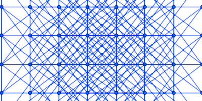
Michael
This is both brilliant and beautiful. But does it suggest an approach to help with the zeros of the Riemann Zeta function?
Thanks for your feedback! I currently can’t think of a way to directly use the derived equations for the Riemann zeta function. It is interesting to note that there exists a (numerically well supported) conjecture for the distribution of the the distance of the zeta function zeros, the Montgomery’s pair correlation conjecture (https://en.wikipedia.org/wiki/Montgomery%27s_pair_correlation_conjecture).
It’s always intriguing and instructive to see how Dr. Trott approaches problems, and manages also to get these beautiful images. Thanks! Definite re-read!
Amazing and appealing!