Two years ago we released Version 13.0 of Wolfram Language. Here are the updates in symbolic and numeric computation since then, including the latest features in 14.0. The contents of this post are compiled from Stephen Wolfram’s Release Announcements for 13.1, 13.2, 13.3 and 14.0.

Calculus

Still Going Strong on Calculus (January 2024)

When Mathematica 1.0 was released in 1988, it was a “wow” that, yes, now one could routinely do integrals symbolically by computer. And it wasn’t long before we got to the point—first with indefinite integrals, and later with definite integrals—where what’s now the Wolfram Language could do integrals better than any human. So did that mean we were “finished” with calculus? Well, no. First there were differential equations, and partial differential equations. And it took a decade to get symbolic ODEs to a beyond-human level. And with symbolic PDEs it took until just a few years ago. Somewhere along the way we built out discrete calculus, asymptotic expansions and integral transforms. And we also implemented lots of specific features needed for applications like statistics, probability, signal processing and control theory. But even now there are still frontiers.

And in Version 14 there are significant advances around calculus. One category concerns the structure of answers. Yes, one can have a formula that correctly represents the solution to a differential equation. But is it in the best, simplest or most useful form? Well, in Version 14 we’ve worked hard to make sure it is—often dramatically reducing the size of expressions that get generated.

Another advance has to do with expanding the range of “pre-packaged” calculus operations. We’ve been able to do derivatives ever since Version 1.0. But in Version 14 we’ve added implicit differentiation. And, yes, one can give a basic definition for this easily enough using ordinary differentiation and equation solving. But by adding an explicit ImplicitD we’re packaging all that up—and handling the tricky corner cases—so that it becomes routine to use implicit differentiation wherever you want:

Another category of pre-packaged calculus operations new in Version 14 are ones for vector-based integration. These were always possible to do in a “do-it-yourself” mode. But in Version 14 they are now streamlined built-in functions—that, by the way, also cover corner cases, etc. And what made them possible is actually a development in another area: our decade-long project to add geometric computation to Wolfram Language—which gave us a natural way to describe geometric constructs such as curves and surfaces:

Related functionality new in Version 14 is ContourIntegrate:

Functions like ContourIntegrate just “get the answer”. But if one’s learning or exploring calculus it’s often also useful to be able to do things in a more step-by-step way. In Version 14 you can start with an inactive integral

and explicitly do operations like changing variables:

Sometimes actual answers get expressed in inactive form, particularly as infinite sums:

And now in Version 14 the function TruncateSum lets you take such a sum and generate a truncated “approximation”:

Functions like D and Integrate—as well as LineIntegrate and SurfaceIntegrate—are, in a sense, “classic calculus”, taught and used for more than three centuries. But in Version 14 we also support what we can think of as “emerging” calculus operations, like fractional differentiation:

College Calculus (June 2022)

Transforming college calculus was one of the early achievements of Mathematica. But even now we’re continuing to add functionality to make college calculus ever easier and smoother to do—and more immediately connectable to applications. We’ve always had the function D for taking derivatives at a point. Now in Version 13.1 we’re adding ImplicitD for finding implicit derivatives.

So, for example, it can find the derivative of x^y with respect to x, with y determined implicit by the constraint
x² + y² = 1:

Leave out the first argument and you’ll get the standard college calculus “find the slope of the tangent line to a curve”:

So far all of this is a fairly straightforward repackaging of our longstanding calculus functionality. And indeed these kinds of implicit derivatives have been available for a long time in Wolfram|Alpha. But for Mathematica and the Wolfram Language we want everything to be as general as possible—and to support the kinds of things that show up in differential geometry, and in things like asymptotics and validation of implicit solutions to differential equations. So in addition to ordinary college-level calculus, ImplicitD can do things like finding a second implicit derivative on a curve defined by the intersection of two surfaces:

In Mathematica and the Wolfram Language Integrate is a function that just gets you answers. (In Wolfram|Alpha you can ask for a step-by-step solution too.) But particularly for educational purposes—and sometimes also when pushing boundaries of what’s possible—it can be useful to do integrals in steps. And so in Version 13.1 we’ve added the function IntegrateChangeVariables for changing variables in integrals.

An immediate issue is that when you specify an integral with Integrate[...], Integrate will just go ahead and do the integral:

But for IntegrateChangeVariables you need an “undone” integral. And you can get this using Inactive, as in:

And given this inactive form, we can use IntegrateChangeVariables to do a “trig substitution”:

The result is again an inactive form, now stating the integral differently. Activate goes ahead and actually does the integral:

IntegrateChangeVariables can deal with multiple integrals as well—and with named coordinate systems. Here it’s transforming a double integral to polar coordinates:

Although the basic “structural” transformation of variables in integrals is quite straightforward, the whole story of IntegrateChangeVariables is considerably more complicated. “College-level” changes of variables are usually carefully arranged to come out easily. But in the more general case, IntegrateChangeVariables ends up having to do nontrivial transformations of geometric regions, difficult simplifications of integrands subject to certain constraints, and so on.

In addition to changing variables in integrals, Version 13.1 also introduces DSolveChangeVariables for changing variables in differential equations. Here it’s transforming the Laplace equation to polar coordinates:

Sometimes a change of variables can just be a convenience. But sometimes (think General Relativity) it can lead one to a whole different view of a system. Here, for example, an exponential transformation converts the usual Cauchy–Euler equation to a form with constant coefficients:

Fractional Calculus (June 2022)

The first derivative of x² is 2x; the second derivative is 2. But what is the derivative? It’s a question that was asked (for example by Leibniz) even in the first years of calculus. And by the 1800s Riemann and Liouville had given an answer—which in Version 13.1 can now be computed by the new FractionalD:

And, yes, do another derivative and you get back the 1^st derivative:

In the more general case we have:

And this works even for negative derivatives, so that, for example, the (–1)^st derivative is an ordinary integral:

It can be at least as difficult to compute a fractional derivative as an integral. But FractionalD can still often do it

though the result can quickly become quite complicated:

Why is FractionalD a separate function, rather than just being part of a generalization of D? We discussed this for quite a while. And the reason we introduced the explicit FractionalD is that there isn’t a unique definition of fractional derivatives. In fact, in Version 13.1 we also support the Caputo fractional derivative (or differintegral) CaputoD.

For the derivative of x², the answer is still the same:

But as soon as a function isn’t zero at x = 0 the answer can be different:

CaputoD is a particularly convenient definition of fractional differentiation when one’s dealing with Laplace transforms and differential equations. And in Version 13.1 we can now only compute CaputoD but also do integral transforms and solve equations that involve it.

Here’s a -order differential equation

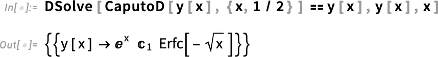
and a -order one

as well as a π^th-order one:

Note the appearance of MittagLefflerE. This function (which we introduced in Version 9.0) plays the same kind of role for fractional derivatives that Exp plays for ordinary derivatives.

Calculus & Its Generalizations (December 2023)

Is there still more to do in calculus? Yes! Sometimes the goal is, for example, to solve more differential equations. And sometimes it’s to solve existing ones better. The point is that there may be many different possible forms that can be given for a symbolic solution. And often the forms that are easiest to generate aren’t the ones that are most useful or convenient for subsequent computation, or the easiest for a human to understand.

In Version 13.2 we’ve made dramatic progress in improving the form of solutions that we give for the most kinds of differential equations, and systems of differential equations.

Here’s an example. In Version 13.1 this is an equation we could solve symbolically, but the solution we give is long and complicated:

&#10005

But now, in 13.2, we immediately give a much more compact and useful form of the solution:

The simplification is often even more dramatic for systems of differential equations. And our new algorithms cover a full range of differential equations with constant coefficients—which are what go by the name LTI (linear time-invariant) systems in engineering, and are used quite universally to represent electrical, mechanical, chemical, etc. systems.

In addition to streamlining “everyday calculus”, we’re also pushing on some frontiers of calculus, like fractional calculus. In Version 13.1 we introduced symbolic fractional differentiation, with functions like FractionalD. In Version 13.2 we now also have numerical fractional differentiation, with functions like NFractionalD, here shown getting the ½^th derivative of Sin[x]:

In Version 13.1 we introduced symbolic solutions of fractional differential equations with constant coefficients; now in Version 13.2 we’re extending this to asymptotic solutions of fractional differential equations with both constant and polynomial coefficients. Here’s an Airy-like differential equation, but generalized to the fractional case with a Caputo fractional derivative:

Line, Surface and Contour Integration (June 2023)

“Find the integral of the function ___” is a typical core thing one wants to do in calculus. And in Mathematica and the Wolfram Language that’s achieved with Integrate. But particularly in applications of calculus, it’s common to want to ask slightly more elaborate questions, like “What’s the integral of ___ over the region ___?”, or “What’s the integral of ___ along the line ___?”

Almost a decade ago (in Version 10) we introduced a way to specify integration over regions—just by giving the region “geometrically” as the domain of the integral:

It had always been possible to write out such an integral in “standard Integrate” form

but the region specification is much more convenient—as well as being much more efficient to process.

Finding an integral along a line is also something that can ultimately be done in “standard Integrate” form. And if you have an explicit (parametric) formula for the line this is typically fairly straightforward. But if the line is specified in a geometrical way then there’s real work to do to even set up the problem in “standard Integrate” form. So in Version 13.3 we’re introducing the function LineIntegrate to automate this.

LineIntegrate can deal with integrating both scalar and vector functions over lines. Here’s an example where the line is just a straight line:

But LineIntegrate also works for lines that aren’t straight, like this parametrically specified one:

To compute the integral also requires finding the tangent vector at every point on the curve—but LineIntegrate automatically does that:

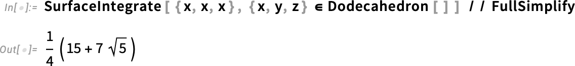
Line integrals are common in applications of calculus to physics. But perhaps even more common are surface integrals, representing for example total flux through a surface. And in Version 13.3 we’re introducing SurfaceIntegrate. Here’s a fairly straightforward integral of flux that goes radially outward through a sphere:

Here’s a more complicated case:

And here’s what the actual vector field looks like on the surface of the dodecahedron:

LineIntegrate and SurfaceIntegrate deal with integrating scalar and vector functions in Euclidean space. But in Version 13.3 we’re also handling another kind of integration: contour integration in the complex plane.

We can start with a classic contour integral—illustrating Cauchy’s theorem:

Here’s a slightly more elaborate complex function

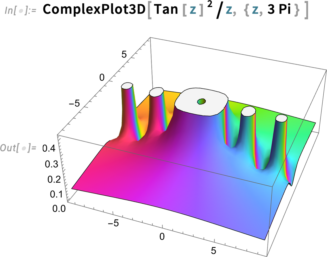
and here’s its integral around a circular contour:

Needless to say, this still gives the same result, since the new contour still encloses the same poles:

More impressively, here’s the result for an arbitrary radius of contour:

And here’s a plot of the (imaginary part of the) result:

Contours can be of any shape:

The result for the contour integral depends on whether the pole is inside the “Pac-Man”:

Matrices & More Math

Finite Fields (January 2024)

In Version 1.0 we had integers, rational numbers and real numbers. In Version 3.0 we added algebraic numbers (represented implicitly by Root)—and a dozen years later we added algebraic number fields and transcendental roots. For Version 14 we’ve now added another (long-awaited) “number-related” construct: finite fields.

Here’s our symbolic representation of the field of integers modulo 7:

And now here’s a specific element of that field

which we can immediately compute with:

But what’s really important about what we’ve done with finite fields is that we’ve fully integrated them into other functions in the system. So, for example, we can factor a polynomial whose coefficients are in a finite field:

We can also do things like find solutions to equations over finite fields. So here, for example, is a point on a Fermat curve over the finite field GF(17³):

And here is a power of a matrix with elements over the same finite field:

More Math—Some Long Awaited (June 2022)

In February 1990 an internal bug report was filed against the still-in-development Version 2.0 of Mathematica:

&#10005

It’s taken a long time (and similar issues have been reported many times), but in Version 13.1 we can finally close this bug!

Consider the differential equation (the Clairaut equation):

What DSolve does by default is to give the generic solution to this equation, in terms of the parameter 𝕔₁. But the subtle point (which in optics is associated with caustics) is that the family of solutions for different values of 𝕔₁ has an envelope which isn’t itself part of the family of solutions, but is also a solution:

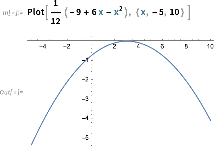
In Version 13.1 you can request that solution with the option IncludeSingularSolutions→True:

And here’s a plot of it:

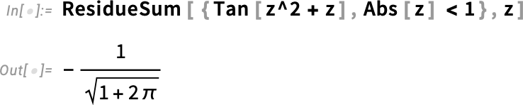
DSolve was a new function (back in 1991) in Version 2.0. Another new function in Version 2.0 was Residue. And in Version 13.1 we’re also adding an extension to Residue: the function ResidueSum. And while Residue finds the residue of a complex function at a specific point, ResidueSum finds a sum of residues.

This computes the sum of all residues for a function, across the whole complex plane:

This computes the sum of residues within a particular region, in this case the unit disk:

Dramatically Faster Polynomial Operations (December 2023)

Almost any algebraic computation ends up somehow involving polynomials. And polynomials have been a well-optimized part of Mathematica and the Wolfram Language since the beginning. And in fact, little has needed to be updated in the fundamental operations we do with them in more than a quarter of a century. But now in Version 13.2—thanks to new algorithms and new data structures, and new ways to use modern computer hardware—we’re updating some core polynomial operations, and making them dramatically faster. And, by the way, we’re getting some new polynomial functionality as well.

Here is a product of two polynomials, expanded out:

Factoring polynomials like this is pretty much instantaneous, and has been ever since Version 1:

But now let’s make this bigger:

There are 999 terms in the expanded polynomial:

Factoring this isn’t an easy computation, and in Version 13.1 takes about 19 seconds:

&#10005

But now, in Version 13.2, the same computation takes 0.3 seconds—nearly 60 times faster:

It’s pretty rare that anything gets 60x faster. But this is one of those cases, and in fact for still larger polynomials, the ratio will steadily increase further. But is this just something that’s only relevant for obscure, big polynomials? Well, no. Not least because it turns out that big polynomials show up “under the hood” in all sorts of important places. For example, the innocuous-seeming object

can be manipulated as an algebraic number, but with minimal polynomial:

In addition to factoring, Version 13.2 also dramatically increases the efficiency of polynomial resultants, GCDs, discriminants, etc. And all of this makes possible a transformative update to polynomial linear algebra, i.e. operations on matrices whose elements are (univariate) polynomials.

Here’s a matrix of polynomials:

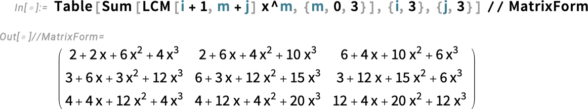
And here’s a power of the matrix:

And the determinant of this:

In Version 13.1 this didn’t look nearly as nice; the result comes out unexpanded as:

Both size and speed are dramatically improved in Version 13.2. Here’s a larger case—where in 13.1 the computation takes more than an hour, and the result has a staggering leaf count of 178 billion

&#10005

but in Version 13.2 it’s 13,000 times faster, and 60 million times smaller:

Polynomial linear algebra is used “under the hood” in a remarkable range of areas, particularly in handling linear differential equations, difference equations, and their symbolic solutions. And in Version 13.2, not only polynomial MatrixPower and Det, but also LinearSolve, Inverse, RowReduce, MatrixRank and NullSpace have been dramatically sped up.

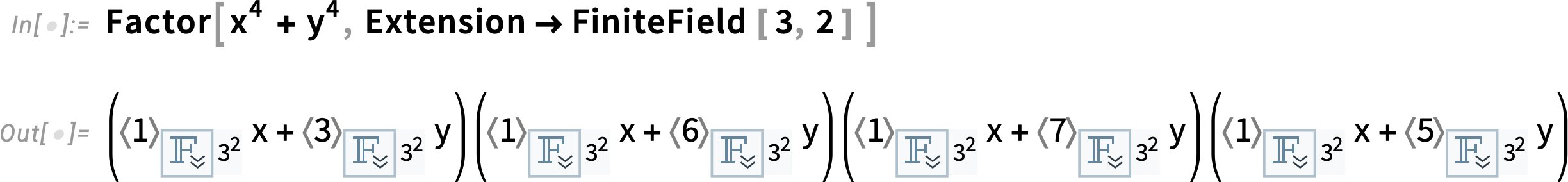
In addition to the dramatic speed improvements, Version 13.2 also adds a polynomial feature for which I, for one, happen to have been waiting for more than 30 years: multivariate polynomial factoring over finite fields:

Indeed, looking in our archives I find many requests stretching back to at least 1990—from quite a range of people—for this capability, even though, charmingly, a 1991 internal note states:

&#10005

Yup, that was right. But 31 years later, in Version 13.2, it’s done!

Another Milestone for Special Functions (June 2023)

One can think of special functions as a way of “modularizing” mathematical results. It’s often a challenge to know that something can be expressed in terms of special functions. But once one’s done this, one can immediately apply the independent knowledge that exists about the special functions.

Even in Version 1.0 we already supported many special functions. And over the years we’ve added support for many more—to the point where we now cover everything that might reasonably be considered a “classical” special function. But in recent years we’ve also been tackling more general special functions. They’re mathematically more complex, but each one we successfully cover makes a new collection of problems accessible to exact solution and reliable numerical and symbolic computation.

Most of the “classic” special functions—like Bessel functions, Legendre functions, elliptic integrals, etc.—are in the end univariate hypergeometric functions. But one important frontier in “general special functions” are those corresponding to bivariate hypergeometric functions. And already in Version 4.0 (1999) we introduced one example of such as a function: AppellF1. And, yes, it’s taken a while, but now in Version 13.3 we’ve finally finished doing the math and creating the algorithms to introduce AppellF2, AppellF3 and AppellF4.

On the face of it, it’s just another function—with lots of arguments—whose value we can find to any precision:

Occasionally it has a closed form:

But despite its mathematical sophistication, plots of it tend to look fairly uninspiring:

Series expansions begin to show a little more:

And ultimately this is a function that solves a pair of PDEs that can be seen as a generalization to two variables of the univariate hypergeometric ODE. So what other generalizations are possible? Paul Appell spent many years around the turn of the twentieth century looking—and came up with just four, which as of Version 13.3 now all appear in the Wolfram Language, as AppellF1, AppellF2, AppellF3 and AppellF4.

To make special functions useful in the Wolfram Language they need to be “knitted” into other capabilities of the language—from numerical evaluation to series expansion, calculus, equation solving, and integral transforms. And in Version 13.3 we’ve passed another special function milestone, around integral transforms.

When I started using special functions in the 1970s the main source of information about them tended to be a small number of handbooks that had been assembled through decades of work. When we began to build Mathematica and what’s now the Wolfram Language, one of our goals was to subsume the information in such handbooks. And over the years that’s exactly what we’ve achieved—for integrals, sums, differential equations, etc. But one of the holdouts has been integral transforms for special functions. And, yes, we’ve covered a great many of these. But there are exotic examples that can often only “coincidentally” be done in closed form—and that in the past have only been found in books of tables.

But now in Version 13.3 we can do cases like:

And in fact we believe that in Version 13.3 we’ve reached the edge of what’s ever been figured out about Laplace transforms for special functions. The most extensive handbook—finally published in 1973—runs to about 400 pages. A few years ago we could do about 55% of the forward Laplace transforms in the book, and 31% of the inverse ones. But now in Version 13.3 we can do 100% of the ones that we can verify as correct (and, yes, there are definitely some mistakes in the book). It’s the end of a long journey, and a satisfying achievement in the quest to make as much mathematical knowledge as possible automatically computable.

Finite Fields! (June 2023)

Ever since Version 1.0 we’ve been able to do things like factoring polynomials modulo primes. And many packages have been developed that handle specific aspects of finite fields. But in Version 13.3 we now have complete, consistent coverage of all finite fields—and operations with them.

Here’s our symbolic representation of the field of integers modulo 5 (AKA ℤ₅ or GF(5)):

And here are symbolic representations of the elements of this field—which in this particular case can be rather trivially identified with ordinary integers mod 5:

Arithmetic immediately works on these symbolic elements:

But where things get a bit trickier is when we’re dealing with prime-power fields. We represent the field GF(2³) symbolically as:

But now the elements of this field no longer have a direct correspondence with ordinary integers. We can still assign “indices” to them, though (with elements 0 and 1 being the additive and multiplicative identities). So here’s an example of an operation in this field:

But what actually is this result? Well, it’s an element of the finite field—with index 4—represented internally in the form:

The little box opens out to show the symbolic FiniteField construct:

And we can extract properties of the element, like its index:

So here, for example, are the complete addition and multiplication tables for this field:

For the field GF(7²) these look a little more complicated:

There are various number-theoretic-like functions that one can compute for elements of finite fields. Here’s an element of GF(5¹⁰):

The multiplicative order of this (i.e. power of it that gives 1) is quite large:

Here’s its minimal polynomial:

But where finite fields really begin to come into their own is when one looks at polynomials over them. Here, for example, is factoring over GF(3²):

Expanding this gives a finite-field-style representation of the original polynomial:

Here’s the result of expanding a power of a polynomial over GF(3²):