As of Today, the Fundamental Constants of Physics (c, h, e, k, NA) Are Finally… Constant!
This morning, representatives of more than 100 countries agreed on a new definition of the base units for all weights and measures. Here’s a picture of the event that I took this morning at the Palais des Congrès in Versailles (down the street from the Château):

An important vote for the future weights and measures used in science, technology, commerce and even daily life happened here today. This morning’s agreement is the culmination of at least 230 years of wishing and labor by some of the world’s most famous scientists. The preface to the story entails Galileo and Kepler. Chapter one involves Laplace, Legendre and many other late-18th-century French scientists. Chapter two includes Arago and Gauss. Some of the main figures of chapter three (which I would call “The Rise of the Constants”) are Maxwell and Planck. And the final chapter (“Reign of the Constants”) begins today and builds on the work of contemporary Nobel laureates like Klaus von Klitzing, Bill Phillips and Brian Josephson.
I had the good fortune to witness today’s historic event in person.

In today’s session of the 26th meeting of the General Conference on Weights and Measures was a vote on Draft Resolution A that elevates the definitions of the units through fundamental constants. The vote passed, and so the draft resolution has been elevated to an international binding agreement.
While the vote was the culmination of the day, this morning we heard four interesting talks (“SI” stands for Système international d’unités, or the International System of Units):
- “The Quantum Hall Effect and the Revised SI,” by Klaus von Klitzing (who is my former postdoc advisor, by the way)
- “The Role of the Planck Constant in Physics,” by Jean-Philippe Uzan
- “Optical Atomic Clocks—Opening New Perspectives on the Quantum World,” by Jun Ye
- “Measuring with Fundamental Constants: How the Revised SI Will Work,” by Bill Phillips
It was a very interesting morning. Here are some pictures from the event:


Yes, these are really tattoos of the new value of the Planck constant.
So why do I write about this? There are a few reasons why I care about fundamental constants, units and the new SI.
Although I am deeply involved with units and fundamental constants in connection with their use in Wolfram|Alpha and the Wolfram Language, I was wearing a media badge today because I have been the science adviser—and sometimes the best boy grip—for the forthcoming documentary film The State of the Unit.
- Units appear in any real-world measurement, and fundamental constants are of crucial importance for the laws of physics. Our Wolfram units team has been collecting data and implementing code over the last decade to help the unit implementation in the Wolfram Language become the world’s most complete and comprehensive computational system of units and physical quantities. And the exact values of the fundamental constants will be of relevance here.
- I have been acting as the scientific adviser for The State of the Unit, which is directed by my partner Amy Young. The documentary covers the story of the kilogram from French Revolutionary times to literally today (November 16, 2018). Together we have visited many scientific institutes, labs, libraries and museums to talk with scientists, historians and curators about the contributions of giants of science such as Kepler, Maxwell, Laplace, Lalande, Planck, de Broglie and Delambre. I have had the fortune to have held in my (gloved) hands the original platinum artifacts and handwritten papers of the heroes of science of the last few hundred years.
Lastly, this blog is a natural continuation of my blog from two years ago, “An Exact Value for the Planck Constant: Why Reaching It Took 100 Years.” This blog discusses in more detail the efforts related to the future definition of the kilogram through the Planck constant.
A lot could be written about the high-precision experiments that made the 2019 SI possible. The hardest (and most expensive) part was the determination of the Planck constant. It involved half a dozen so-called Kibble balances that employ two macroscopic quantum effects (the Josephson and quantum Hall effects) and the famous “roundest objects in the world”: silicon shapes of unprecedented purity that are nearly perfect spheres. The State of the Unit will show details of these experiments and interviews with the researchers.
Before discussing in some more detail the event today and what this redefinition of our units means, let me briefly recall the beginnings of the story.
Something very important for modern science, technology and more happened on June 22, 1799. At the time, this day in Paris was called 4 Messidor an 7 according to the French Revolutionary calendar.
A nine-year journey led by the top mathematicians, physicists, astronomers, chemists and philosophers of France (including Laplace, Legendre, Condorcet, Berthollet, Lavoisier, Haüy, de Borda, Fourcroy, Monge, Prony, Coulomb, Delambre, Méchain) came to a natural end. It was carried out in the middle of the French Revolution; some of the main figures of the story lost their lives in it. And in the end, the metric system was born.
The journey started seriously when, on April 17, 1790, Charles Maurice de Talleyrand-Périgord (Bishop of Autun) presented a plan to the French National Assembly to build a new system of measures based on nature (the Earth) using the decimal system, which was not generally used at this time. At the end of April 1790, the main daily French newspaper Gazette Nationale ou le Moniteur Universel devoted a large article to Talleyrand’s presentation.


The different weights and measures throughout France had become a serious economic obstacle for trade and a means for the aristocracy to exploit peasants by silently changing the measures that were under their control. Not surprisingly, measuring land matters a lot. And so, the Department of Agriculture and Trade was the first to join (in 1790) Talleyrand’s call for new standardized measures.

A few months later in August 1790, the project of building a new system of measures became law. France at this time was still under the reign of Louis XVI.

To make physical realizations of the new measures, the group employed Louis XVI’s goldsmith, Marc-Etienne Janety, to prepare the purest platinum possible at the time.
And to determine the absolute size of the new standards, the length of the meridian was measured with unprecedented precision through a net of triangles between Dunkirk and Barcelona. The so-called Paris meridian goes right through Paris, and actually through the main room (through the middle of the largest window) of the Paris Observatory that was built in 1671.


And to disseminate the new measures, the public had to be convinced of and educated about the advantages of using base 10 for calculations and trade. The National Convention discussed this topic and requested special research about the use of the decimal system (the dissertation shown is from 1793).

The creation of the new measures was not a secret project of scientists. Many steps were publicly announced and discussed, including through posters displayed throughout Paris and the rest of France (the poster shown is from 1793).

The best scientists of the time were employed either part time or full time in the making of the new metric system (see Champagne’s The Role of Five Eighteenth-Century French Mathematicians in the Development of the Metric System and Gillispie’s Science and Polity in France for more detailed accounts). Adrien-Marie Legendre, today better known through Legendre polynomials and the Legendre transform, spent a large amount of time in the Temporary Bureau of Weights and Measures. Here is a letter signed by him on the official letterhead of the bureau:


René Just Haüy, a famous mineralogist, was employed by the government to write a textbook about the new length, area, volume and mass units. His Instruction abrégée sur les mesures déduites de la grandeur de la terre: uniformes pour toute la République: et sur les calculs relatifs à leur division décimale (Abridged Instruction on Measurements Derived from the Size of the Earth: Uniforms for the Whole Republic: and Calculations of their Decimal Division) was first published in 1793 and became, in its 150-page abridged version, a bestseller that was many times republished throughout France.

After nearly 10 years, these efforts culminated in a rectangular platinum bar 1 meter in length, and a platinum cylinder that was 39 millimeters in width and height with a weight of 1 kilogram. These two pieces would become the definitive standards for France and were built by the best instrument makers of the time, Étienne Lenoir and Nicolas Fortin. The two platinum objects were the first and defining realization of what we today call the metric system. A few copies of the platinum meter and kilogram cylinder were made; all have since remained in the possession of the French government. Cities, municipalities and private persons could buy brass copies of the new standards. Here is one brass meter from Lenoir. (The script text under “METRE” reads “Egal a la dixmillionieme partie du quart du Méridien terrestre,” which translates to “Equal to the ten-millionth part of the quarter of the Earth meridian.”)


While the platinum kilogram was a cylinder, the first brass weights for the public were parallelepipeds, also made from brass.

The determination of the length of the meridian was done with amazing effort and precision. But a small error was creeping in, and the resulting meter deviated about 0.2% from its ideal value. (For the whole story of how this happened, see Ken Alder’s The Measure of All Things.)
 ✕
GeodesyData["ITRF00","MeridianQuadrant"] |
Finally came June 22, 1799. Louis Antoine de Bougainville, the famous navigator, had a cold and so could not actively execute his responsibilities at the National Institute. Pierre-Simon Laplace, the immortal mathematician whose name we see still everywhere in modern science through his transform, his operator and his demon, had to take his place. Laplace gave a long speech to the Council of Five Hundred (Conseil des Cinq-Cents) and the Council of Ancients (Counseil des Anciens).
After his speech, Laplace himself, Lefévre-Gineau, Monge, Brisson, Coulomb, Delambre, Haüy, Lagrange, Méchain, Prony and Vandermonde; the Foreign commissionaires Bugge (from Denmark), van Swinden and Aeneae (from Batavia), Tralles (from Switzerland), Ciscar and Pedrayes (from Spain), Balbo, Mascheroni, Multedo, Franchini and Fabbroni (from Italy); and the two instrument makers Lenoir and Fortin took coaches over to the National Archives and deposited the meter and the kilogram in a special safe with four locks. The group also had certified measurements; the certificates were deposited as well.
Something similar has happened today, once again in Paris. Over the last three days, the General Conference on Weights and Measures (CGPM) held its 26th quadrennial meeting. Their first meeting 129 years ago established the meter and kilogram artifacts of 1889 as international standards. The culmination of today’s meeting was a vote on whether the current definition of the kilogram as a material artifact will be replaced by an exact value of the Planck constant. Additionally, the electron charge, the Boltzmann constant and the Avogadro constant will also get exact values (the speed of light has had an exact value since 1983).

Every few years, new values (with uncertainties) have been published for the fundamental constants of physics, by CODATA. Back in 1998 the value of the electron charge was  . The latest published value is
  . This morning, it was decided that soon it will be exactly
  and it will always be this, forever.
But what exactly does it mean for a fundamental constant to have an exact value? It is a matter of the defining units. When a unit (like a coulomb) is exactly defined, then determining the value of the charge of an electron becomes a precision measurement task (a path followed for 100+ years since Millikan’s 1909 droplet experiments). When the value of the elementary charge is exactly defined, realizing 1 coulomb becomes a task of precision metrology.
The situation is similar for the other constants: give the constant an exact defined value, and use this exact value to define the unit. Most importantly, the Planck constant will get an exact value that will define the kilogram, the last unit that is still defined through a manmade artifact.
Over the past decades, scientists have measured the Planck constant, the electron mass, the Boltzmann constant and the Avogadro constant through devices that were calibrated with base units of kilogram, ampere, kelvin and mole. In the future, the values of the constants will be exact numbers that define the units. The resulting system is the natural revision of the SI, more simply called the metric system. To emphasize the new, enlarged dependence on the fundamental constants of physics, this revision has been called the “new SI” (or, sometimes, the “constants-based SI”).
Today, a revolution in measurement happened. Here is a slide from Bill Phillips’ talk:

Today’s vote completes a process foreseen by James Clerk Maxwell in 1871. This process started in 1892 when Michelson (known for the famous Michelson–Morley experiment for the nonexistence of the aether) connected the length of a meter with the wavelength of a cadmium line. The process advanced more recently in 1983 when the speed of light changed from a measured value to an exact constant of size  meters per second that today defines the meter.
Reading through Laplace’s speech from June 22, 1799, is interesting. Here are five paragraphs from his speech:
“We have always felt some of the advantages that the uniformity of weights and measures will have. But from one country to another and in the very interior of each country, habit, prejudices were opposed on this point to any agreement, any reform.
“It was therefore necessary to find the principle in Nature, that all nations have an equal interest in observing and choosing it, so far as its convenience could determine all minds.
“This unity, drawn from the greatest and most invariable of bodies which man can measure, has the advantage of not differing considerably from the half-height and several other measures used in different countries; common opinion.
“Overcoming a multitude of physical and moral obstacles, they have been acquitted with a degree of perfection of which we have had no idea until now. And in securing the measure they were asked, they have collected and demonstrated in the figure of the Earth the irregularity of its flattening, truths as curious as new.
“But if an earthquake engulfed, if it were possible that a frightful blow of lightning would melt the preservative metal of this measure, it would not result, Citizen Legislators, that the fruit of so many works, that the general type of measures could be lost for the national glory, or for the public utility.”
Many parallels could be drawn to today. International trade without a common system of units is unimaginable. As in the 1790s, dozens of scientists around the world have labored for decades to make as precise as possible with current technology measurements of the Planck and other constants, a precision unimaginable even 50 years ago. And like 219 years ago, defining the new units has been an international effort. And although the platinum meter and kilogram have endured well and fortunately no earthquake or lightning has hit them, the new definitions are truly resistant against any natural catastrophe, and are even suitable for sharing with aliens.
Laplace addressed the Councils one week after van Swinden (one of the foreign delegates) had published the scientific and technical summary of all operations that were involved in the creation of the metric system.

Once the new system was established, its use would be mandated by the French government. Here is a letter from the end of 1799, written from the interior minister François de Neufchâteau to the Northern Department of France ordering the use of the new measures. Despite the government’s efforts, the metric system would not displace old measures for 40 years in France (we can blame this largely on Napoléon).

And one of the last professions to adopt the new measures was medicine. Only in January of 1802 was it even considered.

In contrast, the proposed revised SI was accepted today, and will take effect in just 185 days on May 20, 2019, World Metrology Day.
The 2019 SI will come in much more quietly. Some newspapers have occasionally reported on the experiments. But just as with the original SI, today not everybody is 100% happy with the new system, e.g. some chemists do not like decoupling the mole from the kilogram.
The story that leads to today covers the making of an exact replica of the kilogram from the late 1790s in the 1880s, as well as a slightly improved version of the platinum meter bar. This kilogram, also called the International Prototype of the Kilogram (IPK), is still today the standard of the unit of mass. As such, it is today the last artifact that is used to define a unit.
The metric system in its modern form is de facto used everywhere in science, technology, commerce, trade and daily life. All US-customary measures are defined and calibrated through the metric standards. As a universal measurement standard, it was instrumental in quantifying and quantitatively describing the world.
“À tous les temps, à tous les peuples” (“For all times, for all people”) were the words that were planned for a commemorative medal that was suggested on September 9, 1799 (23 fructidor an 7), to be minted to honor the creation of the metric system. (Similar to the metric system itself, the medal was delayed by 40 years.) Basing our units on some of the most important fundamental constants of physics bases them on the deepest quantifying properties of our universe, and at the same time defines them for all times and for all people.
So what exactly is the new SI? The metric system started with base units for time, length and mass. Today, SI has seven base units: the second, the meter, the kilogram, the ampere, the kelvin, the mole and the candela. The so-called SI Brochure is the standard document that defines the system. The currently active definitions are:
s: the second is the duration of  periods of the radiation corresponding to the transition between the two hyperfine levels of the ground state of the caesium-133 atom
m: the meter is the length of the path traveled by light in a vacuum during a time interval of 1/299 792 458 of a second
kg: the kilogram is the unit of mass; it is equal to the mass of the IPK
A: the ampere is that constant current that, if maintained in two straight parallel conductors of infinite length and of negligible circular cross-sections and placed one meter apart in a vacuum, would produce between these conductors a force equal to 2 ×  newtons per meter of length
K: the kelvin, the unit of thermodynamic temperature, is the fraction 1/273.16 of the thermodynamic temperature of the triple point of water
mol: the mole is the amount of substance in a system that contains as many elementary entities as there are atoms in 0.012 kilograms of carbon-12
cd: the candela is the luminous intensity, in a given direction, of a source that emits monochromatic radiation of frequency 540 ×  hertz and that has a radiant intensity in that direction of 1/683 watt per steradian
Some notes to these official definitions:
- The kilogram is defined relative to a human-made artifact, the IPK. The IPK is a better platinum-quality replica of the original late-18th-century kilogram made by Fortin with the platinum from Janety.
- The definition of the ampere that involves infinitely long, infinitesimally thick wires is not very practical.
- The definition of the kelvin uses a material macroscopic substance, namely water.
- With its reference to the kilogram, the definition of the mole is strictly coupled to the kilogram.
The proposed definitions of the new SI, based on fixed values of the fundamental constants, are available from the draft of the next edition of the SI Brochure. First the importance and values of the constants are postulated.
The SI is the system of units in which:
- the unperturbed ground-state hyperfine transition frequency of the caesium-133 atom
 is
is  Hz
Hz - the speed of light in vacuum c is
 m/s
m/s - the Planck constant
 is
is  J s
J s - the elementary charge
 is
is 
- the Boltzmann constant
 is
is 
- the Avogadro constant
 is
is 

- the luminous efficacy of monochromatic radiation of frequency
 hertz
hertz  is 683 lm/W
The definitions now read as follows:
s: The second, symbol s, is the SI unit of time. It is defined by taking the fixed numerical value of the caesium frequency  , the unperturbed ground-state hyperfine transition frequency of the caesium-133 atom, to be
  when expressed in the unit Hz, which is equal to
  .
.
m: The meter, symbol m, is the SI unit of length. It is defined by taking the fixed numerical value of the speed of light in vacuum  to be
to be  when expressed in the unit
  , where the second is defined in terms of the caesium frequency
  .
.
kg: The kilogram, symbol kg, is the SI unit of mass. It is defined by taking the fixed numerical value of the Planck constant h to be  when expressed in the unit J s, which is equal to kg
  , where the meter and the second are defined in terms of c and
  .
.
A: The ampere, symbol A, is the SI unit of electric current. It is defined by taking the fixed numerical value of the elementary charge e to be  , when expressed in the unit C, which is equal to A s, where the second is defined in terms of
  .
.
K: The kelvin, symbol K, is the SI unit of thermodynamic temperature. It is defined by taking the fixed numerical value of the Boltzmann constant k to be  when expressed in the unit J
  , which is equal to kg
  , where the kilogram, meter and second are defined in terms of h, c and
  .
.
mol: The mole, symbol mol, is the SI unit of amount of substance. One mole contains exactly  elementary entities. This number is the fixed numerical value of the Avogadro constant,
  , when expressed in the unit
  and is called the Avogadro number.
cd: The candela, symbol cd, is the SI unit of luminous intensity in a given direction. It is defined by taking the fixed numerical value of the luminous efficacy of monochromatic radiation of frequency 540 ×  Hz,
Hz,  , to be 683 when expressed in the unit lm
  , which is equal to cd sr
  , or cd sr

 , where the kilogram, meter and second are defined in terms of h, c and
  .
.
Compared with the early 2018 SI definitions, we observe:
- Any reference to material artifacts or macroscopic objects has been eliminated.
- The definitions are all based on fundamental constants of physics.
- The building up of the base units is much more recursive than it was before.
- The mole has become an independent unit (de facto a dimensional counting unit).
- The ampere had the practically unrealizable definition through infinite wires, but is now conceptually and for small currents through single-electron pumps already practically reduced to a counting-like operation.
- The 200+-year-old idea to base our units on nature has been implemented on a much deeper conceptual level. To connect units with fundamental constants, we need two more ingredients: fundamental constants and physical laws. The ontological connection between units and fundamental constants has to go through physical laws, concretely these three famous laws of physics: a)
 ; b)
; b)  for the definition of the kilogram through the Planck constant; and c)
  for defining the kelvin through the Boltzmann constant. For the kilogram, to connect the Planck constant
  with a mass, one follows de Broglie and equates
  with
with  to arrive at
  , which connects mass with the Planck constant.
Determining the values of the constants to a precision allows us to supersede the old definitions, and thus ensures that the associated changes in the values of the units will have no disruptive influence on any measurement is a remarkable success of modern science.
Two hundred twenty years ago, not everybody agreed on the new system of units. The base (10 or 12) and the naming of the units were frequent topics of public discussion. Here is a full-page newspaper article with a suggestion of a slightly different system than the classic metric system.

Now let’s come back to the fundamental constants of physics.
From a fundamental physics point of view, it is not a priori clear that the fundamental constants are constant over great lengths of time (billions of years) and distance in the universe. But from a practical point of view, they seem to be as stable as anything could be.
What is the relative popularity of the various fundamental constants? The arXiv preprint server, with its nearly one million physics preprints, is a good data source to answer this question. Here is a breakdown of the frequencies with which the various fundamental constants are explicitly mentioned in the preprints. (The cosmological constant only became so popular over the last three decades, and it is a constant current unsuitable for defining units.)

There is a lot of philosophical literature, theoretical physics and numerology literature about fundamental constants and their meaning, values and status within the universe (or multiverse) and so on. Why do the constants have the values they have? Is humankind lucky that the constants have the values they have (e.g. only minute changes in the values of the constants would not allow stars to form)? Fundamental constants allow many back-of-the-envelope calculations as they govern all physics around us. Here is a crude estimation for the height of a giraffe in terms of the electron and proton mass, the elementary charge, the Coulomb constant  , the gravitational constant
  and the Bohr radius
  :
:
![Subscript[m, e]](https://content.wolfram.com/sites/39/2018/11/2Novimg65.png "Subscript [m, e]") ✕
|
(Subscript[m, e]/Subscript[m, p])^(1/20) ((κ e^2)/(G Subscript[m, p]^2))^(3/10) Subscript[a, 0]//UnitConvert[#,"Feet"]&
This is not the place to review this literature of the theory and uses of fundamental constants, or to contribute to it. Rather, let’s use the Wolfram Language to see how fundamental constants can be used in actual computations.
Fundamental constants are tightly integrated into the computational subsystem of the Wolfram Language that deals with units, measures and physical laws. The fundamental constants are in the upper-left yellow box of the network graphic:


These are the five constants from the new SI and their current values expressed in SI base units:
|
✕
siConstants = {Quantity[1, "SpeedOfLight"],
   Quantity[1, "PlanckConstant"], Quantity[1, "ElementaryCharge"],
   Quantity[1, "BoltzmannConstant"], Quantity[1, "AvogadroConstant"]};
|
 ✕
Grid[Transpose[{siConstants/. 1->None, UnitConvert[siConstants,"SIBase"]}],Dividers->Center,Alignment->Left]//TraditionalForm
|
Physical constant are everywhere in physics. We use the function FormulaData to get some examples.
") ✕
siConstantNames=Alternatives @@ (Last/@ siConstants) |
 ✕
formulas=Select[{#,FormulaData[#] /.
Quantity[a_,b_. "ReducedPlanckConstant"^exp_.] :>
   Quantity[a/(2Pi),b "PlanckConstant"^exp]}&/@ FormulaData[],
MemberQ[#, siConstantNames, ∞]&];
|
The left column shows the standard names of the formulas, and the right column shows the actual formulas. The symbols (E, T, …) are all physical quantity variables of PhysicalQuantity[...,...]). Here are the shortest formulas that contain a physical constant:
 ✕
makeGrid[data_] := Grid[{Column[Flatten[{#}]],#2}&@@@
Take[ SortBy[data,LeafCount[Last[#]]&], UpTo[12]],
Dividers->Center,Alignment->Left]
|
![makeGrid[formulas]](https://content.wolfram.com/sites/39/2018/11/3Novimg6.png "makeGrid[formulas]") ✕
makeGrid[formulas] |
And here are the formulas that contain at least three different physical fundamental constants:
 ✕
makeGrid[Select[formulas, Length[Union[Cases[#,siConstantNames, ∞]]]>2&]] |
One of the many entity types included in the Wolfram Knowledgebase is fundamental constants. There is some discussion in the literature of what exactly constitutes a constant. Are any dimensional constants really physical constants, or are they “just” artifacts of our units? Do only dimensionless coupling constants, typically around 26 in the standard model of particle physics, describe the fabric of our universe? We took a liberal approach and also included derived constants in our data as well as anthropologically relevant values, such as the Sun’s mass, that are often standardized by various international bodies. This gives a total of more than 210.
 ✕
EntityValue["PhysicalConstant","EntityCount"] |
Expressed in SI base units, the constants span about 160 orders of magnitude. Converting all constants to Planck units gives dimensionless values for the constants and allows for a more honest and faithful representation.
 ✕
toPlanckUnits[u_?NumberQ ]:=Abs[u]

toPlanckUnits[Quantity[v_,u_] ]:=  Normal[UnitConvert[Abs[v] u/.
{"Meters" -> 1/Quantity[1, "PlanckLength"], "Seconds" -> 1/Quantity[1, "PlanckTime"],
"Kilograms" -> 1/Quantity[1, "PlanckMass"], "Kelvins"->1/Quantity[1, "PlanckTemperature"],
"Amperes" ->1/ Quantity[1,"PlanckElectricCurrent"]},"SIBase"] /.
("Meters"|"Seconds"|"Kilograms"|"Kelvins"|"Amperes"):>1]
|
 ✕
constantsInPlanckUnits=SortBy[Cases[{#1, toPlanckUnits@UnitConvert[#2,"SIBase"]}&@@@
EntityValue["PhysicalConstant",{"Entity", "Value"}],{_,_?NumberQ}],Last];
|
 ✕
ListLogPlot[MapIndexed[Callout[{#2[[1]],#1[[2]] }, #[[1]]]&,constantsInPlanckUnits],
                        PlotStyle -> PointSize[0.004],AspectRatio->1,GridLines->{{},{1}}]
|
Because the values of the constants span many orders of magnitude, one expects the first digits to obey (approximately) Benford’s law. The yellow histogram shows the digit frequencies of the constants, and the blue shows the theoretical predictions of Benford’s law.
 ✕
Show[{Histogram[{First[RealDigits[N@#2]][[1]]&@@@constantsInPlanckUnits,
WeightedData[Range[9], Table[Log10[1+1/d],{d, 9}]]},{1},"PDF",
Ticks -> {None, Automatic}, AxesLabel -> {"first digit", "digit frequency"}],Graphics[Table[Text[Style[k, Bold],{k, 0.03}],{k,9}]]}]
|
Because of the different magnitudes and dimensions, it is not straightforward to visualize all constants. The function FeatureSpacePlot allows us to visualize objects that lie on submanifolds of higher-dimensional spaces. In the following, we take the magnitudes and the unit dimensions of the constants into account. As a result, dimensionally equal or similar constants cluster together.
 ✕
constants=Select[{#1, UnitConvert[#2,"SIBase"]}&@@@
EntityValue["PhysicalConstant", {"Entity","Value"}],Not[StringMatchQ[#[[1,2]], (___~~("Jupiter"|"Sun"|"Jupiter")~~___)]]&];
|
 ✕
siBaseUnits={"Seconds","Meters","Kilograms","Amperes","Kelvins","Moles","Candelas"};
|
 ✕
constantsData=Cases[{ Log10[Abs[N@QuantityMagnitude[#2] ]],
N@Normalize[Unitize[Exponent[QuantityUnit[#2],siBaseUnits]]],
#1}&@@@(constants /.{"Steradians"->1} ), {_?NumberQ,_,_}];
|
 ✕
allSIConstants=(Entity["PhysicalConstant",#]&/@
{"AvogadroConstant","PlanckConstant","BoltzmannConstant","ElementaryCharge",
 "SpeedOfLight","Cesium133HyperfineSplittingFrequency"});
|
The poor Avogadro constant is so alone. :-) The reason for this is that not many named fundamental constants contain the mole base unit.
 ✕
(FeatureSpacePlot[Callout[(1 + #2/100) #2,Style[#3, Gray]]&@@@ constantsData , ImageSize ->1600,Method -> "TSNE",ImageMargins->0,PlotRangePadding->Scaled[0.02], AspectRatio->2,PlotStyle->PointSize[0.008]]/.((#->Style[#, Darker[Red]])&/@allSIConstants) )// Show[#, ImageSize -> 800]& |

They are (not mutually exclusively) organized in the following classes of constants:
 ✕
EntityClassList["PhysicalConstant"] |
As much as possible, each constant has the following set of properties filled out:
 ✕
EntityValue["PhysicalConstant","Properties"] |
Most properties are self-explanatory; the Lévy‐Leblond class might not be. A classic paper from 1977 classified the constants into three types:
Type A: physical properties of a particular object
Type B: constants characterizing whole classes of physical phenomena
Type C: universal constants
Here are examples of constants from these three classes:
 ✕
typedConstants=With[{d=EntityValue["PhysicalConstant",{"Entity", "LevyLeblondClass"}]},
Take[DeleteCases[First/@ Cases[d, {_,#}],Entity["PhysicalConstant","EarthMass"]],UpTo[10]]&/@ {"C","B","A"}];
|
 ✕
TextGrid[Prepend[PadRight[typedConstants,Automatic,""]//Transpose,
Style[#,Gray]&/@ {"Type C", "Type B", "Type A"}],Dividers->Center]
|
Physicists’ most beloved fundamental constant is the fine-structure constant (or the inverse, with an approximate value of 137). As it is a genuinely dimensionless constant, it is not useful for defining units.
 ✕
EntityValue[Entity["PhysicalConstant","InverseFineStructureConstant"],{"Value","StandardUncertainty"}] //InputForm
|
There are many ways to express the fine-structure constant through other constants. Here are some of them, including the von Klitzing constant  , the impedance of the vacuum
  , the electron mass
  , the Bohr radius
  and some others:
 ✕
(Quantity[None,"FineStructureConstant"]==#/.Quantity[1,s_String]:> Quantity[None,s])&/@ Entity["PhysicalConstant", "FineStructureConstant"]["EquivalentForms"]//Column//TraditionalForm |
This number puzzled and continues to puzzle physicists more than any other. And over the last 100 years, many people have come up with conjectured exact values of the fine-structure constant. Here we retrieve some of them using the "ConjecturedValues" property and display their values and the relative differences to the measured value:
 ✕
alphaValues=Entity["PhysicalConstant","FineStructureConstant"]["ConjecturedValues"]; |
 ✕
TextGrid[{Row[Riffle[StringSplit[StringReplace[#1,(DigitCharacter~~__):>""],RegularExpression["(?=[$[:upper:]])"]]," "]],
"Year"/.#2,"Value"/.#2,NumberForm[Quantity[100 (N[UnitConvert[("Value"/.#2)/α,"SIBase"]]-1),"Percent"],2]}&@@@
DeleteCases[alphaValues,"Code2011"->_],Dividers->All,
Alignment->Left]
|
Something of great importance for the fundamental constants is the uncertainty of their values. With the exception of the fundamental constants that now have defined values, fundamental constants are measured, and every experiment has an inherent uncertainty. In the Wolfram Language, any number can be precision tagged, e.g. here is π to 10 digits:
 ✕
π10=3.1415926535`10 |
The difference to π is zero within an uncertainty/error of the order  :
:
 ✕
Pi-π10 |
Alternatively, one can use an interval to encode an uncertainty:
 ✕
π10Int = Interval[{3.141592653,3.141592654}]
|
 ✕
Pi-π10Int |
When using precision-tagged, arbitrary-precision numbers as well as intervals in computations, the precision (interval width) is computed, and does represent the precision of the result.
In the forthcoming version of the Wolfram Language, there will be a more direct representation of numbers with uncertainty, called Around (see episode 182 of Stephen Wolfram’s “Live CEOing” livestream).
For a natural (one could say canonical) use of this function, we select five constants that have exact values in the new SI:
 ✕
newSIConstants=ToEntity/@ {c,h,e,k,Subscript[N, A]}
|
These five fundamental constants are (of course) dimensionally independent.
 ✕
DimensionalCombinations[{},
 IncludeQuantities -> {Quantity[1, "SpeedOfLight"],
   Quantity[1, "PlanckConstant"], Quantity[1, "ElementaryCharge"],
   Quantity[1, "BoltzmannConstant"], Quantity[1, "AvogadroConstant"]}]
|
If we add  and
and  , then we can form a two-parameter family of dimensionless combinations.
 ✕
DimensionalCombinations[{},
 IncludeQuantities ->
  Join[{Quantity[1, "SpeedOfLight"], Quantity[1, "PlanckConstant"],
    Quantity[1, "ElementaryCharge"], Quantity[1, "BoltzmannConstant"],
     Quantity[1, "AvogadroConstant"]}, {Quantity[1,
     "MagneticConstant"], Quantity[1, "ElectricConstant"]}]]
|
Let’s take the Planck constant. CODATA is an international organization that every few years takes all measurements of all fundamental constants and calculates the best mutually compatible values and their uncertainties. (Through various physical relations, many fundamental constants are related to each other and are not independent.) For instance, the values from the last 10 years are:
 ✕
hValues={#1, {"Value","StandardUncertainty"}/.#2}&@@@Take[Entity["PhysicalConstant", "PlanckConstant"]["Values"], 5]
|
PS: The strange-looking value of  is just the reduced fraction of the previously stated new exact value for the Planck constant when the value is expressed in units of J·s.
 ✕
662607015/100000000*10^-34 |
Here are the proposed values for the four constants  ,
,  ,
,  and
and  :
:
 ✕
{hNew,eNew,kNew,NAnew}=("Value"/.("CODATA2017RecommendedRevisedSI"/.#["Values"]))&/@ Rest[newSIConstants]
|
Take, for instance, the last reported CODATA value for the Planck constant. The value and uncertainty are:
 ✕
hValues[[4,2]] |
We convert this expression to an Around.
 ✕
toAround[{value:Quantity[v_,unit_], unc:Quantity[u_,unit_]}] := Quantity[Around[v,u], unit]

toAround[HoldPattern[Around[Quantity[v_,unit_],Quantity[u_,unit_]]]]:= Quantity[Around[v,u],unit]

toAround[{v_?NumberQ, u_?NumberQ}] := Around[v,u]

toAround[pc:Entity["PhysicalConstant",_]] := EntityValue[pc,{"Value","StandardUncertainty"}]
|
 ✕
toAround[hValues[[4,2]]] |
Now we can carry out arithmetic on it, e.g. when taking the square root, the uncertainty will be appropriately propagated.
 ✕
Sqrt[%] |
Now let’s look at a more practical example: what will happen with  , the permeability of free space after the redefinition? Right now, it has an exact value.
![["Value"]](https://content.wolfram.com/sites/39/2018/11/3Novimg54.png "[\"Value\"]") ✕
Entity["PhysicalConstant", "MagneticConstant"]["Value"] |
Unfortunately, keeping this value after defining h and e is not a compatible solution. We recognize this from having a look at the equivalent forms of  .
.
![["EquivalentForms"]](https://content.wolfram.com/sites/39/2018/11/3Novimg56.png "[\"EquivalentForms\"] width=") ✕
Entity["PhysicalConstant", "MagneticConstant"]["EquivalentForms"] |
The second one shows that keeping the current value would imply an exact value for the fine-structure constant. The value would be this number:
|
✕
UnitConvert[2*(1/e^2)*(1α)*(1h)*(1/c),"SIBase"] |
 ✕
With[{e=eNew,h=hNew},
           π/2500000N/(A)^2 (c e^2)/(2h) ]
|
 ✕
N[1/%, 10] |
What one must do instead is consider the equation:
![]()
… as the defining equation for  , and this shows that in the new SI
  will have a relative uncertainty equal to the uncertainty of the fine-structure constant.
 ✕
With[{e=eNew,h=hNew,α=toAround[Entity["PhysicalConstant", "FineStructureConstant"]]},
α UnitConvert[(2h)/(c e^2),"SIBase"]] //toAround
|
Before ending this blog (once in Versailles, I should have some nice French pastry in a café rather than yammer on for another ten pages about fundamental constants), let me quickly mention some fun number-theoretic consequences of the exact values for the constants.
With the constants of the new SI having exact values (rational numbers in a mathematical sense) in SI base units, compound expressions that are rational functions of these constants will unavoidably also have rational values.
Using the "EquivalentForms" property, we can quickly select some such constants:
 ✕
Grid[Select[Flatten[Function[{p, ps}, {Text[CommonName[p]],#}&/@ ps] @@@
DeleteMissing[EntityValue["PhysicalConstant",{"Entity","EquivalentForms"}],1,2],1], DeleteCases[Cases[#[[2]],_String, ∞],siConstantNames]==={}&&FreeQ[#,Pi,{0, ∞}]&],Dividers->All,Alignment->Left]
|
Let’s have a look at the two constants from the macroscopic quantum effects that were used in the process of determining the value of the Planck constant: the Josephson constant and the von Klitzing constant.

Here is a photo of von Klitzing’s talk. Note the many digits given for the von Klitzing constant.
We start with the Josephson constant:
 ✕
With[{e=eNew,h=hNew},(2e)/h ] //UnitConvert[#,"SIBase"]&
|
When the value is expressed in SI base units, the corresponding decimal number has a leading number of 4 and then a repeating sequence of digits of length 6.3 million.
 ✕
Short[rdJ=RealDigits[21362351200000000000000/44173801], 3] |
This long period even has the first seven digits of the Planck constant and the elementary charge value inside (which is, of course, pure numerology).
 ✕
{SequencePosition[rdJ[[1,2]],{6,6,2,6,0,7,0}],
SequencePosition[rdJ[[1,2]],{1,6,0,2,1,7,6}]}
|
Now let’s have a look at the von Klitzing constant with a value (well known from the quantum Hall effect) of about 25.8  :
:
 ✕
FromEntity[Entity["PhysicalConstant", "VonKlitzingConstant"]] |
 ✕
UnitConvert[%,"SIBase"]//UnitSimplify |
The digits of the magnitude in base 10 are trivial to obtain:
 ✕
RealDigits[QuantityMagnitude[%]] |
 ✕
With[{e=eNew,h=hNew},h/e^2 ] //UnitSimplify
|
As a rational number, what properties does it have?
Before answering this question, as a reminder about decimal fractions, let’s digress for a moment and have a look at the period of a fraction  . Using the function RealDigits, we can easily find the period for rational numbers (with small denominators). Here we use the example
  :
:
 ✕
RealDigits[5/49] |
|
✕
periodLength[r_] := If[MatchQ[#,{_Integer ..}],0,Length[Last[#]]]&[RealDigits[r][[1]]]
|
 ✕
periodLength[5/49] |
Formatting the decimal digits with an appropriate length shows the period visually.
 ✕
N[5/49,800] //Pane[#,{350,300}]&
|
Generically, the period can have length  . Here is a plot of the period of all
  for
for  :
:
 ✕
Graphics3D[{EdgeForm[],Table[Cuboid[{p-1/2, q-1/2,0},{p+1/2, q+1/2,periodLength[p/q]}],{p,100},{q,100}]}, Axes -> True,BoxRatios->{1,1,1/2},AxesLabel->{"p","q","period"}]
|
If the period length is  , then
  is prime.
![Select[Table[{q, periodLength[1/q]}](https://content.wolfram.com/sites/39/2018/11/3Novimg85.png "Select[Table[{q, periodLength[1/q]}") ✕
Select[Table[{q,periodLength[1/q]},{q,2,100}], #[[2]]>=#[[1]]-1&]
|
![Select[Table[{q, periodLength[2/q]}](https://content.wolfram.com/sites/39/2018/11/3Novimg86.png "Select[Table[{q, periodLength[2/q]}") ✕
Select[Table[{q,periodLength[2/q]},{q,2,100}], #[[2]]>=#[[1]]-1&]
|
![Select[Table[{q, periodLength[3/q]}](https://content.wolfram.com/sites/39/2018/11/3Novimg87.png "Select[Table[{q, periodLength[3/q]}") ✕
Select[Table[{q,periodLength[3/q]},{q,100}], #[[2]]>=#[[1]]-1&]
|
So what is the period of the von Klitzing constant? Here is a small function that calculates the period of a proper fraction less than 1 in base 10. The function returns the numbers of nonrepeating and repeating digits, respectively.
 ✕
decimalDigitCount[b_Rational?(# < 1&)] := Module[{q= FactorInteger[Denominator[b]],r,m,c}, If[Complement[First /@ q, {2, 5}] === {},{Max[Last /@ q], 0}, {c=Max[Last /@ Cases[q, {2 | 5, _}]];If[c == -∞, 0, c], r=Times @@ Power@@@Cases[q, {Except[2|5], _}]; m/.(Solve[Mod[10^m,r]==1∧m>0,m,Integers]/._C->1)[[1]]}]]
|
The period is about 344.2 trillion. (This means don’t try to call RealDigits on the quantity magnitude of the von Klitzing constant in the new SI base units.)
 ✕
decimalDigitCount[vK=55217251250000000000/2139140853713163-25812] |
As a quick check, we implement a function that calculates the  th digit of a rational number in base
  .
.
 ✕
NthDigit[ r:Rational[p_Integer?Positive, q_Integer?Positive]?(0 < # < 1&),
                 n_Integer?Positive, base_Integer?Positive] :=
Floor[base Mod[p PowerMod[base, n - 1, q], q]/q]
|
Indeed, the period of the decimal fraction of the fractional part of the von Klitzing constant in SI base units is that large:
|
✕
periodvK=344229188825340; |
 ✕
Table[NthDigit[vK,j, 10],{j, 20}]
|
 ✕
Table[NthDigit[vK,j+periodvK, 10],{j, 20}]
|
This concludes my “short” report from Versailles, where just hours ago the basis for the metric system was officially redefined (and, in turn, the US customary system of weights and measures, because it is tightly coupled to the SI). Exactly 80,135 days after two precious platinum artifacts were delivered to the French National Archives, the values of five fundamental constants (the speed of light, the Planck constant, the elementary charge, the Boltzmann constant and the Avogadro constant) were delivered in the form of five rational numbers to mankind. Millions of digital copies of these numbers will exist on the internet (and in a few human memories), and no earthquake or lightning could ever delete them all. The new definitions could last for a long, long time, as artifacts (which themselves were once predicted to last 10,000 years) are no longer involved. Today’s vote does not mean that nothing will ever change again. At the bottom of the chain of definitions, the unit of time—the second—is defined through about nine billion radiation cycles. Replacing this definition with some higher-frequency radiation, and thus a larger, more precisely countable number, might be the next change. But a new definition of the second will still be based on a fundamental constant of physics.
Download this post as a Wolfram Notebook.

Great article Michael!
Its interesting to think that WRI is continuing the scientific odyssey which began with the French Revolution. Viva La Science! Perhaps we should celebrate by cutting off the heads of all those string theory losers who have been clogging up the top positions in Physics departments.
Michael
What will we do if it turns out c or G varied since the Big Bang?
Very simple. The new definitions are much, much more immutable than the previous ones. Too many orders of magnitude. This is the point. It is obvious to me that the job of BIPM will be never finished. Already meter has had its second definition since getting rid of the meter based on a bar. This will go on forever and ever.
Think over all once again… ;-)
Nice post Michael! However, I am curious about one thing. You write, that in the new SI, “2. The definitions are all based on fundamental constants of physics”. In what form is Avogadro’s number a fundamental constant of physics? Is it not an arbitrary integer that was chosen for historical reasons? It is not an observable constant of our physical world like the speed of light, but is a dimensionless measure that is part of mathematics, just like Pi. And even if SI considers counting measures, why is it not the integer 1 that became the dimensionless unit of “amount”? Then mole should be a derived, secondary quantity. What am I missing?
István, this is a good question and one that I have seen and heard repeatedly! The Avogadro constant is considered a fundamental constants of physics. But compared to many of the other fundamental constants of physics that come from the micro-world, the Avogadro constant connects micro-world with the macro-world. In the latter we have for instance the classical gas laws that uses moles. Determining how many particles make one mole has a long history going back to Loschmidt’s 1865 determination. (Avogadro himself never determined ‘his’ number and the name only was used in 1909 by Perrin the first time.)
More pragmatically, the fact that there is a formula that connects the Planck constants, the Rydberg constant, the speed of light, and the fine structure constant (all of which one would naturally see as fundamental constants) does contain the Avogadro constant shows that it is a fundamental constant of physics.
For a more in-depth discussion, see Wheatley’s paper (http://precedings.nature.com/documents/5138/version/1/files/npre20105138-1.pdf%3Forigin%3Dpublication_detail), especially section 6
Great you got to see your postdoc advisor, and witness the “happy marriage” of high science and the fundamental (constants) with metrology!
Very, very interesting! Thank you, Michael!
I guess I’m curious about one thing. It’s not exactly clear to me why the old standard of mass – a platinum bar sitting in an enclosed container – is slowly changing its mass over time. What is exactly is going wrong? Surely the platinum bar wasn’t wet on the surface, and is now losing moisture? It can’t be that platinum is somehow “vaporizing” at room temperature, so why is the mass changing? I’m just curious. Being from the “old school”, I do like the look and feel of standards that I can actually touch – even if I will never be allowed to touch the platinum mass standard. Anyway, the new system of force measurement seems intriguing. Very ingenious.
Hello Pete and thanks for your question. Indeed the evaporation rate of platinum at room temperature is extremely small. So, the weight loss (measured with respect to other kilogram artifacts) is not due to a loss of platinum or iridium atoms. One is not totally sure today what actually causes the weight loss. There are various conjectures out there. One being that in the early years the cylinder absorbed mercury from a thermometer that was stored in the same safe and now this mercury comes out again. Also the first decades the cylinder was stored at lower air pressure. This might have initiated an internal diffusion process of hydrogen.
I must question your first statement “Any reference to material artifacts or macroscopic objects has been eliminated.” Aren’t Cs-133 and light material artifacts ? Clearly much of the dependence on “macroscopic objects” has been eliminated – as is appropriate. But have we gone too far ? I am particularly disturbed by the definition of the mole- what the hell is a “dimensional counting unit”. Why not just base it on Pi, which is functionally more suitable ? Thank you for your very comprehensive and well researched article. rlp
Hi Richard! Thanks for submitting your questions. A Cs-133 atom is definitely a material object. But it is not an artifact, meaning a man-made macroscopic object. Indeed, the new definition of the mole stands out as it is technically indeed a counting unit. And maybe in the future we will have a proper unit (say ‘ent’) for a single countable microscopic object (meaning it is indistinguishable from other and obeys a Bose or Fermi statistics).
Let me leave a second comment. Suppose we were trying to convey our system of units to an extra-terrestrial entity. I think our system would be near undecipherable. Does that say something ?
I think you refer to the many digits and the large/small exponents of the powers of 10 in the values of the constants. I think there are two things that aliens would infer from this:
a) Our approximate size and weight. The fact that we define our base units in such a way that we normally have to deal with numbers sau from 0.001 to 1000 in most cases.
b) The long sequence of digits indicate to aliens that once we had artifacts as standards and we aimed for a smooth transition from the artifacts to the constants-based definitions.
Michael. Greetings and thanks for you reply. Very interesting. I do want to finish with one thought. I understand that the world of physics has switched gears and will not measure mass by using a force standard. But let’s use our imagination for a minute. And really – this is not so imaginative. It appears that the platinum mass standard (the old standard) had problems with mercury contamination and gas absorption. These things could be fixed – they could be re-engineered. A new mass standard made from ultra-pure platinum could be manufactured. How would be very it? By taking very tiny samples and running them through a mass spectrometer. With great efforts, we could probably produce a platinum bar with exception purity. After that – put this bar inside a container with an ultra-high vacuum, and run it through many temperature cycles. So in this way, any absorbed gases will be removed. Finally, and this is the interesting thought, lets imagine we have a solid bar of perfectly pure platinum, perhaps weighing 1.00000000000005 kg. Don’t quote me on the exact number of zeros (but it’s a lot). These days we have instruments like the Atomic Force Microscope that can actually be used to “etch” the surface on solids on an atomic scale. So we could literally knock off platinum atoms, in very tiny amounts. Hence the final weight of the platinum bar could be reduced until we get to … 1.00000000000000000. OK, now we do need to ask … how many zero’s after the decimal point? The atomic weight of platinum is 195.09 gram. Avogadros number is 6.02472 x 10^23. Doing the division gives the mass of one platinum atom as … 3.24 x 10^-22. So in principle we could “micro-machine” that platinum bar down to an accuracy of 22 zeros after the decimal point. That is an incredibly accurate standard of mass. It is probably not possible for the platinum to be a cylinder. A simple cube or sphere might be sufficient. But maybe … just maybe … an extraordinary standard of mass is achievable. Perhaps there is some other limit that stops us from doing this, I don’t know. I just think that it is interesting. Maybe in the future, physicists might again need to have a real mass standard built from actual atoms. In that case, I believe that it is possible. OK … well thanks very much for the whole article which was very, very interesting!
Thanks for your detailed reply. You mention a couple of very interesting points.
The Planck constant serves as a definition of a kilogram and through a Kibble balance also as a primary realization. But this is a quite expensive process and currently doable at a precision of the order 10^-8.
At a practical level metal cylinders of various types stored in various gases and in vacuum will be used for comparisons. See Estefanía de Mirandés’ https://www.bipm.org/cc/CCM/Allowed/16/04C_Status-ERMS.pdf> talk for details.
While practically mass is often measured through actual force comparisons, the abstract definition through the Planck constant makes no direct reference to a force. So in principle one could come up with force-free mass measurements.
Your idea to make a very precise mass standard through actually counting is definitely a very appealing one. Such an approach has been tried at the PTB (see http://iopscience.iop.org/article/10.1088/0026-1394/47/3/005). There are unfortunately two problems with this. a) Even if one could count say 1 billion platinum atoms per second (which is already far outside of current technology) one would need about 90 million years to accumulate a mass of 1 kg and b) in the experiments carried out one makes from time to time a mistake in counting or an atom gets lost and this error was in the order 10^-5 or larger. To make single platinum atoms one needs to heat the metal and then the high thermal velocity of the toms makes them hard to collect. So, the counting approach is great conceptually but currently not realizable.
Sorry. Above comment. The 2nd sentence should say … I understand that the world of physics has switched gears and will *now* measure mass by using a force standard.
Very good website you have here but I was wondering if you knew of any community
forums that cover the same topics discussed here?
I’d really like to be a part of online community where I can get suggestions from
other experienced people that share the same interest.
If you have any suggestions, please let me know.
Kudos!
Hi Jerrold. If you haven’t already, you should check out the Wolfram Community website. There are a large selection of topics to explore (https://community.wolfram.com/groups).
First of all, I want to thank you for the very very interesting article.
I would really like to become a member of the forum, where I could get acquainted with the opinion of qualified specialists on this topic. Please advise the Internet address.
The latter concerns the recommended value of relative uncertainty in measuring fundamental constants.
To calculate the value of relative uncertainty, modern statistical methods and supercomputers are used. In addition, at each stage of evaluating the results an expert analysis of the obtained data is carried out. This means using your own intuition, knowledge and experience of a specialist (personal philosophical inclinations). Such a situation does not exclude the presence of a biased statistical expert motivated by personal convictions or preferences. It should be noted that the method of relative uncertainty for determining the accuracy of measurement does not indicate the direction in which the true value of the fundamental physical constant can be found. In addition, it includes an element of subjective judgment.
Do you consider it permissible to approach this issue from a strictly theoretical position?
I would like to draw your attention to the fact that in contrast to the statistical expert CODATA methods, I proposed a theoretically sound approach based on information theory / B. Menin, h, k, NA: Evaluating the Relative Uncertainty of Measurement, American Journal of Computation and Applied Mathematics, 8 (5) (2018) 93-102, http://article.sapub.org/10.5923.j.ajcam. 20180805.02.html./. The theoretically calculated relative uncertainties agree very well with the CODATA recommendations. In addition, the calculations are very simple, carried out in a short time and are available even to such a non-professional as me. I would be grateful if you express your opinion on this issue.
Respectfully
Boris
Both the fine structure constant and Planck’s constant have their bases in Thomas precession. Proofs with extremely high correspondence between the theory, models, and experimental results are given in my article ‘Thomas precession is the basis for the structure of matter and space’ at this link https://www.researchgate.net/publication/328572809_Thomas_Precession_is_the_Basis_for_the_Structure_of_Matter_and_Space?_sg=CmQxvEb9ANN2jCZJ7KK4xuFYJgnlb2xlNTRwfVEkMt9WwCkbrYXPBW1KxHEE_mqmI4WSRi7wrI7jZIm1D-FHx4VA5jb_42g6Zc2OKA66.oTNnRmCeua3oFFs5h5hi2U07REEMR2f1fmAT1gJwd9leEuyFikScMfzPIC0oMlCNhpcmBajbo0gp9y-fuzGIpg