While working with SARS-CoV-2 genetic data in the Wolfram Data Repository, we noticed that there was frequently only a relative handful of differences compared with the overall size of the sequences. This allowed us a number of interesting opportunities for further processing.

First of all, with so much in common, the sequences could be aligned more rapidly by checking for large identical regions and then reducing the alignment task to the sections with differences. Let’s look at an example. First, we’ll gather a BioSequence for the reference SARS-CoV-2 from a Wolfram Data Repository we maintain for this:

Engage with the code in this post by downloading the Wolfram Notebook

&#10005

Next, we will arbitrarily pick another SARS-CoV-2 sequence:

&#10005

The resource function AlignNearlyIdenticalSequences allows us to find an alignment between these sequences rather quickly:

&#10005

The alignment itself shows the similarities and differences between the two sequences. Given that these sequences are rather long with broad sections of similarity, it seems helpful to extract just the differences. To accomplish this, we created the resource function AlignmentToPositionDifferences.

AlignmentToPositionDifferences converts an alignment to a list of positions with replacement rules. These can be interpreted as where particular changes might be made in the first sequence to yield the second sequence:

&#10005

These position differences have many different possible uses. For example, with a number of similar sequences, you might want to align them to a reference. You can then gather the sequences that have similar differences or use them as features in other analyses and potentially combine them with dates or geographic data. A handful of these applications can be seen in the Analysis section at the SARS-CoV-2 genetics data repository.

Beyond its analytical uses, this is also a great method for compression. Given a reference sequence and a number of variant sequences, we can reduce the size of the variant sequences by nearly an order of magnitude over a raw string representation:

&#10005

&#10005

To restore a sequence from these positional differences, we’ve developed the ReconstituteSequenceFromReferenceDifferences resource function. Given the difference and the reference sequence, the function reconstitutes the other sequence:

&#10005

When working with sequence differences for analysis, there are always two different kinds of possible analysis: where there might be a difference versus where there must be a difference. This occurs because the sequencing process does not always produce exact results about which base is at a particular position. Fortunately, there is a broadly adopted standard for which additional letters are used to represent potential choices among specific bases. These letters are called degenerate letters:

&#10005

If you’re working with cases where there might be a difference between two sequences, you can use alignment differences directly:

&#10005

If you’re interested in where they must be different, however, the resource function RemoveDegenerateSequenceDifferences will reduce the differences to those without a degenerate match, eliminating positional differences when no disparity remains:

&#10005

This is a practical concern, as many SARS-CoV-2 sequences have a number of degenerate differences with the reference sequence:

&#10005

When degenerate letter matches are accounted for, the differences are reduced considerably:

&#10005

Visualizing a DNA Sequence

One common way to visualize DNA and RNA sequences is by using frequency chaos game representation (FCGR). For this purpose, there is the FCGRImage resource function:

&#10005

Gauging Proximities between Genetic Sequences

Another useful thing to do with a set of genomes is to show them in a way that indicates the relative distances between pairs. We will show two ways to do this. Here we download a set of coronaviruses, which can take up to a minute or so, to see which ones seem closest to SARS-CoV-2:

&#10005

Now get the short names and the genome strings:

&#10005

Use the resource function PhylogeneticTreePlot to create a dendrogram from these sequences:

&#10005

Another visualization is as a dimension-reduced point set. We use the resource function MultidimensionalScaling (hereafter MDS) for this purpose. First we need to create vectors representing the genome sequences, and then reduce them to three dimensions. There are many ways to do this. We will employ the process used in PhylogeneticTreePlot.

We start by creating the FCGR image data arrays. We use a Fourier discrete cosine transform to remove high-frequency details, then use a common method from principal component analysis (PCA) to get vectors of length 40:

&#10005

The final step is to use MDS to reduce to 3D:

&#10005

You’ll see that the SARS and the SARS-CoV-2 families each cluster closely and both separate well from the various other coronaviruses.

Working with Preexisting Proximity Resources

Throughout COVID-19, there has been a number of great analyses with results derived from data not available to the general public. These proximity results include the Newick trees published by Nextstrain. Newick is a format for expressing phylogenetic trees in terms of nested branches with distances. Here is a trivial example shown with an imported result and dendrogram using the ImportNewickString and NewickDendrogram resource functions:

&#10005

&#10005

We observe that the nodes b and c are at the same depth, given that they are the same overall distance from the root (4 + 1 and 5, respectively).

This Nextstrain COVID-19 data is provided via a link at the bottom of the Nextstrain global page. Once that data is downloaded, it’s ready to be imported:

&#10005

&#10005

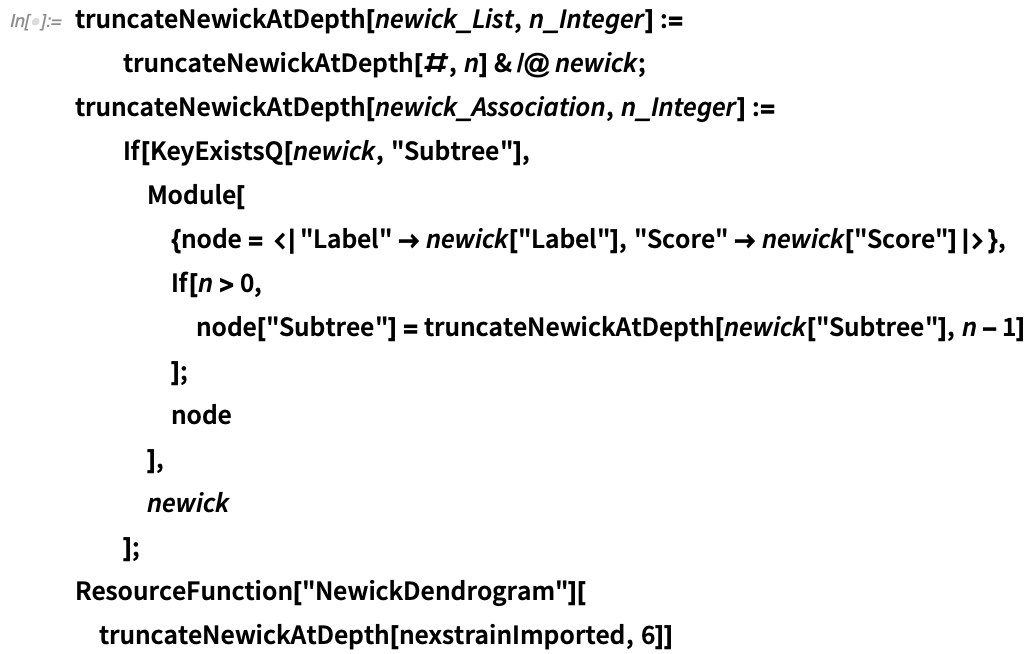
This tree is too large to display in a single dendrogram. Instead, we can show the tree up to a given level of nesting, truncated recursively from the root:

&#10005

In this tree, all of the non-strain nodes are of the form NODE_<number>. If we’d like to look further into the tree, we can find such a node and similarly display a truncated subset of it:

&#10005

Of course, this is just a small taste of the analysis that is possible for the Newick format or the Nextstrain data and would be a good area for further extension.

Identifiers and Further Information

Accessions and other identifiers are useful for more than gathering their sequences and also offer links to supporting information, such as related PubMed entries:

&#10005

Sometimes there can be a fair number of these resources:

&#10005

Supporting Metadata

In addition to providing resources for working directly with sequences, sometimes it is also useful to operate on the metadata for functions. For example, BioSequenceTranslate will accept arguments determining what translation table is used. All of the typical ones are provided through the "GeneticTranslationTable" entities:

&#10005

These translations are provided in both expansive and terse forms, which are easier to edit and more compact to use, respectively:

&#10005

&#10005

You may have occasion, however, to use a custom translation and to want to move between the more expansive and condensed forms as you switch between editing and use. The resource function NCBITranslationTableConvert switches between these formats:

&#10005

&#10005

Beyond Genetic Sequences: Protein Sequences

Gene sequences are not the only kind of biomolecular sequence with supporting functionality. The resource function PDBImport allows you to access protein properties and diagrams from the RCSB Protein Data Bank identifier:

&#10005

An Invitation

The Wolfram Function Repository isn’t only for Wolfram employees; we review and publish submissions by and for our users. One user-submitted item, DNAAlignmentPlot, produces a nifty plot of the results from sequence alignment:

&#10005

There is so much more yet to do. If you find yourself with sequence processing functionality that you’d like to share, even if only for your own later convenience, consider submitting it to the Function Repository. We would be delighted to help deliver it to whomever happens to need it.