Musing about Rectangular Bar Magnets
(This is the third post in a three-part series about electrostatic and magnetostatic problems involving sharp edges.)
In the first blog post of this series, we looked at magnetic field configurations of piecewise straight wires. In the second post, we discussed charged cubes and orbits of test particles in their electric field. Today we will look at magnetic systems, concretely, mainly at a rectangular bar magnet with uniform magnetization.
As a warm-up, let’s use Wolfram|Alpha for the visualization of the magnetic induction of a magnetizable ball in a constant magnetic field. While this is a standard exercise for calculations involving spherical harmonic expansions, it is very convenient to have the magnetic field inside and outside the ball ready at one’s fingertips.

We define the magnetic induction in a cross section through the center of the sphere parallel to the outer field.

Using the StreamPlot function, we can quickly and conveniently show the magnetic field direction in a cross section of the sphere.

And here is a plot of the magnitude of the field strength.

What is the energy stored in magnetic induction of the sphere outside the sphere? We use the total magnetic field and subtract the external field and integrate the magnetic energy density in spherical coordinates.

Now let’s come to the rectangular bar magnet. To visualize the field of a bar magnet, we first need a closed-form expression for the magnetic field strength. Again we use Wolfram|Alpha through the WolframAlpha[] function to obtain the needed formulas. Already the scalar magnetic vector potential is a pretty large expression; we display a scaled-down version.

As a side note, the last expression is intimately related to the above used potential of a cube. The scalar magnetic vector potential equals the derivative of the electric potential with respect to z. We also now use the more general form for arbitrary edge lengths a, b, and c to be able to model a bar magnet of realistic edge length ratios. Here is the corresponding expression for the magnetic field ![]() (x, y, z). (While elementary, a closed-form expression for the magnetic field around a rectangular bar magnet was only published in 2004 by Engel-Herbert and Hesjedal.)
(x, y, z). (While elementary, a closed-form expression for the magnetic field around a rectangular bar magnet was only published in 2004 by Engel-Herbert and Hesjedal.)

For the following examples, we choose a bar magnet of dimensions 1 x 1 x 2. Plotting the magnetic field strength in the vicinity of an edge (in the x = 0 plane) shows a pronounced singularity of the magnetic field strength along the edge.

Calculating a series expansion around the center of an edge shows that the type of the singularity of the field strength is logarithmic.

Magnetic materials with smooth boundaries do not exhibit arbitrarily large field strength. The existence of the edges on the cube boundary causes the logarithmic singularities in the field strengths. Practically, one cannot measure arbitrarily high field strength at the edge of a bar magnet because of the discrete atomic nature of the magnet. But the fields near an edge of a magnet are used to produce larger magnetic fields; see for instance the two papers by Samofalov ([1] [2]).
Compared with magnetic field value at the face center, in a distance one millionth of the size of the magnet from the corner, the field strength is about four times larger.

A look at the magnetic field in the cross section of the magnet shows the upper and lower faces as the source of the field. (These are quantitative correct versions of the typical qualitative textbook sketches for the magnetic lines of a bar magnet.)

Here is a slightly different view—a 3D plot of the surfaces of constant magnitude of the ![]() -field.
-field.

While the magnetic field ![]() has sources, the magnetic induction
has sources, the magnetic induction ![]() is source-free (remember the Maxwell equation div
is source-free (remember the Maxwell equation div ![]() = 0). We obtain the magnetic field
= 0). We obtain the magnetic field ![]() by adding the magnetization
by adding the magnetization ![]() to the magnetic field
to the magnetic field ![]() . (Here we use all dimensions set to 1; of course, in SI units the magnetic field strength and the magnetic induction have different units.) The right plot shows the field lines, which now are closed. The field lines of
. (Here we use all dimensions set to 1; of course, in SI units the magnetic field strength and the magnetic induction have different units.) The right plot shows the field lines, which now are closed. The field lines of ![]() and
and ![]() coincide outside the magnet.
coincide outside the magnet.

Using the function LineIntegralConvolutionPlot, we can make a visualization of the field lines quite similar to the images one obtains using a real magnet and iron filings.

We know that the normal components of ![]() and the tangential components of
and the tangential components of ![]() should be continuous functions across the boundary of a magnet. We can quickly verify this for the fields along the right vertical and top face of the magnet in the equatorial plane.
should be continuous functions across the boundary of a magnet. We can quickly verify this for the fields along the right vertical and top face of the magnet in the equatorial plane.


The magnetic induction within the magnet is approximately constant in direction and magnitude. Here is a closed form for the value at the center.

The next two plots show the magnetic field and the magnetic induction over the magnet.


We can even calculate the series expansion at the center of the magnet to get a quantitative estimation of how constant the magnetic induction is at the center for symbolic edge lengths. The first nonvanishing contributions for the deviation from a constant field value are of second order. (Meaning the constancy is less than that of a Helmholtz coil discussed in the first blog post of this series.)

We will end this blog post with an interactive example of two rectangular bar magnets. We assume both magnets are in a plane, and we can move them freely around. What does the resulting magnetic field look like? And, more important for many applications (such as for magnetic drug delivery), what is the force on a small magnetizable particle in the field of two magnets? Because the force will be proportional to ![]() |
|![]() |^2, an interesting and, in the first moment, counterintiuitive situation can arise:
|^2, an interesting and, in the first moment, counterintiuitive situation can arise:
The force always points toward the magnet, either to the North Pole or to the South Pole, but never away from it. By properly aligning two magnets, we can have a point outside of the two magnets where the magnetic induction ![]() vanishes due to the two superimposed fields. On the side of this point toward the magnets, the force on a test particle is toward one of the two magnets, but on the other half-space, the force is away from the magnets. This effect, that the combined magnetic field of two simple magnets can be used for pushing a magnetic object away from the magnets, is of great relevance for controlled magnetic drug delivery in the human body. The following interactive demonstration lets us study the position of these points of vanishing field strength by changing the positions, orientations, and pole strengths of the two magnets.
vanishes due to the two superimposed fields. On the side of this point toward the magnets, the force on a test particle is toward one of the two magnets, but on the other half-space, the force is away from the magnets. This effect, that the combined magnetic field of two simple magnets can be used for pushing a magnetic object away from the magnets, is of great relevance for controlled magnetic drug delivery in the human body. The following interactive demonstration lets us study the position of these points of vanishing field strength by changing the positions, orientations, and pole strengths of the two magnets.


We end here and let the reader continue, for instance, by calculating the trajectories of a magnetic point dipole ![]() in the field of a rectangular bar magnet. The force on the dipole is given either by
in the field of a rectangular bar magnet. The force on the dipole is given either by ![]() ~ grad(
~ grad(![]() .
.![]() ) or through
) or through ![]() ~ (
~ (![]() .
.![]() )
)![]() ).
).
Many more interesting and novel calculations can be carried out for charged cubes and bar magnets, for example, what is the equivalent to Coulomb’s (Newton’s law) of attraction between two cubes, which leads to some interesting and challenging six-dimensional integrals. We will continue our cube investigations in a later blog post.
Download this post as a Computable Document Format (CDF) file.


Wow. Just discovered these posts and I am very impressed. FWIW, I was thinking of how I might use Mathematica to visualize problem in a college EM course I’m teaching, and these demos go a long way towards answering my problem :)
Please keep them coming.
Dear Michael, compliments for the graphics.
Nice expressions for bar magnets are given by Yonnet, (search terms Yonnet cuboidal). Field, forces and torque are covered by several authors. See also http://mathematica.stackexchange.com/questions/38063/contourplot3d-for-a-3d-vector-contour-plot.
wow that is so very cool
The call \[Phi]MagnetizableBallData =
WolframAlpha[
“magnetizable ball in a magnetic field”, \
{{“Properties:PhysicalSystems”, 1}, “Input”}] for wolfram alpha did not work.
It is trying to get the input from the first field in the ‘physical systems’ pod of the wolfram output. That pod data is here…
\[Phi]MagnetizableBallData =
ReleaseHold[
Hold[Piecewise[{{OverVector[
Subscript[B,
0]] + (2*Quantity[1, “MagneticConstant”]*OverVector[M])/3,
Sqrt[x^2 + y^2 + z^2] (3*(-Quantity[1, “MagneticConstant”] + \[Mu])*
OverVector[Subscript[B, 0]])/(Quantity[1,
“MagneticConstant”]*(2*
Quantity[1, “MagneticConstant”] + \[Mu])),
OverVector[n] :> {x, y, z}/Sqrt[x^2 + y^2 + z^2],
OverVector[m] :> (4*Pi*R^3*OverVector[M])/3}]
I did this by doing the natural language search for ‘magnetizable ball in a magnetic field’
It still didn’t work! I get output that looks similar (but much more complex) and the graphics don’t work.
Link to non-working code that I think I executed well.
https://drive.google.com/file/d/0B-Qyee_GJfdiZFRpenV4Q3AyWDQ/view?usp=sharing
(its just a .PNG screenshot of what I got).
It is frustrating how hard it is to get what you actually want with the wolframalpha[] method.
Thank you for your comment! We changed some of the naming, so the new call that does not produce that result is below:
WolframAlpha[“magnetizable ball in a magnetic field”, \
{{“Electromagnetism:PhysicalSystem”, 1}, “Input”}]