3D Charges and Configurations with Sharp Edges
In my last blog post, we looked at various examples of electrostatic potentials and magnetostatic fields. We ended with a rectangular current loop. Electrostatic and magnetostatic potentials for squares, cubes, and cuboids typically contain only elementary functions, but the expressions themselves are often quite large compared with simple systems with radial symmetry. In the following, we will discuss some 3D charge configurations that have sharp edges.
Let’s start with a charged 2D rectangle in 3D space. Again, the potential is an elementary function that contains a few logarithms.
![]()

We name the computable form for further computational use, and we define the scaled electrical potential for a rectangle.
![]()


Near the charge itself, the potential decreases linearly with the distance from the potential.
![]()

At a corner, we have a slightly more complicated distance dependence.
![]()

The following graphic of the constant electric-field-magnitude surface reflects the shape of the charged rectangle.


Having at hand the closed form of the potential of a single rectangle, we can use the superposition principle to calculate the electric field distribution of an arrangement of multiple rectangles. In the absence of a jack, we will have a look at a sphere-in-a-box. The box we model as five squares; we consider an already open box and omit the top square (the lid). We will use the same charge for each face of the box.

Here are the equipotential surfaces of the resulting open box (we show part of the box cut open).


We now add a sphere of total charge Qs at the vertical symmetry line of the box and calculate the resulting potential and electric field strength.

To visualize the resulting field distribution, we show field lines originating from the faces of the box and ending on the sphere.

We implement the visualization as a Manipulate. This allows us to change the charge and size of the box and to move it in and out. If the sphere’s charge compensates or exceeds the box’s charge, all field lines end at the sphere. Otherwise some field lines will escape to infinity.


The natural generalization of a charged square is a charged cube. Fortunately Wolfram|Alpha knows the electrostatic potential of a uniformly charged cube; it is already quite a formidable expression that is neither easy to remember nor easy to derive.
![]()

A charged cube is a nice nontrivial model of a charge distribution that isn’t trivial, yet can still be used for exact calculations. We will do some of these in the remaining part of this post.
We specialize to a unit cube (edge length 1) extending from -1/2 to 1/2 along the three coordinate axes. In the chosen units we have ΔV = -4π.
 extending from -1/2 to 1/2 along the three coordinate axes")

Just to convince ourselves that this long result is really correct, let’s quickly compare with the numerical result from explicit integration of Poisson’s equation with the Green’s function.
![]()

Here are the values of the potential in closed form and shown numerically at geometrically exceptional points. Because the expression for the potential is often undefined at the faces and edges itself (of the form 0/0), we use Limit to calculate the potential values.


The complete agreement between the symbolically and numerically derived values gives us confidence that the model is correct.
It is instructive to plot the potential and its derivatives along a line connecting the center of the cube and the center of a face. The potential itself is a smooth function, the field strength (first derivative of the potential) has a kink at the surface of the cube, and the second derivative of the potential (via Poisson’s equation related to the charge density) is discontinuous at the surface of the cube. (Note that the Laplacian of the potential is proportional to the charge density, and in the following plot we show just the second derivative with respect to z. As a result the yellow line is not piecewise constant.)


Let us explore the electric field of a charged cube in more detail.
![]()
It’s a pretty large expression, measuring nearly 700 KB in size.


Here is a plot of the field strength and direction in the equatorial plane.


The maximum field strength occurs at the centers of the faces. This is not unexpected, as the potential of a charged ball exhibits its maximum also on the surface of the ball.


Comparing the field strengths at the face centers, edge centers, and corners shows that the face centers indeed are the points of the largest magnitude of the field strengths.
![]()

![]()

![]()
![]()
![]()
![]()
Plotting the constant field-magnitude surface in 3D in one octant gives the following picture. (The surface of the charged unit cube is shown in light yellow.)


While most equi-field strength surfaces look like parts of a single deformed sphere-like surface, near the edge of the cube some more interestingly shaped equi-field strength surfaces exist that are topologically not a sphere.


The images above show approximately spherical equipotential and equi-field strength surfaces near the center of the cube and far away from the cube. From far, far away, a charged cube looks in first order as a point charge. To quantify the deviation from the charge of a point charge, we carry out a multipole expansion.
We could just expand the Green’s function for large distances and integrate term-wise over a cube. This shows that far away the potential has the form ((V(r))~(|r|-1) + c5|r|-5 + c7 c5|r|-7 + …. The absence of the lower order terms proportional to r-2, r-3, and r-4 explains why for large distances the equipotential surfaces appear so spherical.


Alternatively, we can use the well-known multipole expansion in spherical coordinates.

This yields the same result, here demonstrated for the l = 4 term.


))/(480 (x^2 + y^2 + z^2)^(9/2))")
Before leaving our explorations of an electric field of a charged cube (or the mathematically equivalent problem of a gravitational field of a massive cube), we should have a quick look at the equivalent of the Kepler problem: the motion of a test particle in the field of a charged cube, as pioneered by Liu, Baoyin, and Ma and recently studied in more detail by Chappel, Iqbal, and Abbott. We can easily do this using the numerical differential equation solving capabilities of Mathematica. To quickly solve the equations of motions, we define a compiled version of the electric field strength of our charged unit cube.

To easily see and explore the orbits, we use a Manipulate. Here we assume the cube to be penetrable. The orbits around a point mass are well-known Kepler’s ellipses. We leave it to the reader to investigate if there are closed orbits around a cube, and for which initial conditions such closed orbits exist.


Most real-world charged cubes are not penetrable (and a charged plasma in the form of a cube is difficult to keep in this shape), so a more realistic model would model the cube as a solid, and a test charge would be reflected when it hits one of its faces. We can make the test charge bounce at the cube relatively straightforwardly by adding the "EventLocator" method of NDSolve. We initiate a bounce if the trajectory would cross a face, and we assume a totally elastic reflection process.


A bouncing test charge revolving around a charged cube ends our second blog post about charge distributions with edges. Not that there is not more to be calculated. For instance, what is a closed form for the total electrostatic self-energy of a charged cube Σ▫ = ∫R3ρ(r)V(r)dr? Here is the numerical result.
![]()
![]()
Carrying out the integration over the potential over the unit cube is challenging, and the conjectured exact form is:
![]()
![]()
![]()
Download this post as a Computable Document Format (CDF) file.


Fantastic! Thanks for the fascinating read; I can’t wait for the next installment. I liked the use of EventLocator in NDSolve, that could have many far reaching applications. None of the standard textbooks would even consider these types of nice examples because of the computational difficulty, but with Mathematica and Michael Trott, you can get pretty far.
Really really neat blog. Short elegant code packs a punch. I am mightily impressed a) that Wolframalpha can calculate the electric potential of a charged cube and b) how easily anyone can reuse the result. But I wonder whether can Mathematica calculate the force between TWO charged cubes, a la Fornberg http://www2.maths.ox.ac.uk/chebfun/examples/quad/html/TwoCubes.shtml?
Hi Rich –
Thank you for the question. You can see Michael’s response here: https://blog.wolfram.com/2012/10/23/calculating-the-energy-between-two-cubes/
Finally!
101 years after the rise of cubism in paintings, we now have cubism in physics. What would Picasso have said? Newton’s law of gravitation for cubes, not just spheres–how exciting. Imagine: cubic expoplanets somewhere in outer space.