Stabilized Inverted Pendulum
Can you balance a ruler upright on the palm of your hand? If I concentrate, I can just barely manage it by constantly reacting to the small wobbles of the ruler. This challenge is analogous to a classic problem in the field of control systems design: stabilizing an upside-down (“inverted”) pendulum.
One of the best things about Mathematica is that it makes specialist areas like control systems accessible to non-specialists. This lets you freely combine and develop new ideas without needing to be an expert in everything. It also makes Mathematica a great platform for learning and exploring new areas.
Using the new control systems features (one of several new application areas integrated into Mathematica 8), I’ve been experimenting with models of stabilized inverted pendulums. I’m no expert in control theory, but you’ll see that one doesn’t need to be.

Inverted pendulums arise as models of many real-world systems: Segway vehicles (rocking forward and backward), bicycles (rocking side-to-side), unicycles (both), rockets (during liftoff), and even skyscrapers.
In this post we’ll model a single inverted pendulum on a moving cart, shown above, and use the new control systems functionality to stabilize it. In later posts in this series, we’ll generalize the problem, looking at double (and triple and quadruple) pendulums, pendulums in 3D, and more.
First we need to simulate the pendulum-and-cart system, and then we can try to determine a “control” force f(t) that will move the cart to keep the pendulum balanced upright.
Assuming the pendulum arm is uniform (so its center of mass is at d/2), ignoring friction, and using dimensionless units in which the gravitational acceleration g = 1, the model pendulum-and-cart system shown above satisfies this pair of differential equations:
![]()
(We will derive these equations programmatically for a more general case in the next post. To see an outline of how to derive this case directly, download the Computable Document Format [CDF] file.)
In this post, we’ll explore the concrete case m = c = d = 1:
![]()
Using NDSolve, we can immediately simulate this system from a slightly off-center initial condition θ(0) = π/2 – 0.1. We’ll initially use no control force: f(t) = 0; that is, we make no attempt to move the cart to keep the pendulum upright.

Here’s an animation of the solution:
![]()
(For the definition of the function AnimatePendulum, download the CDF file.)
We can combine the above two steps into a handy function that animates the system for any control force f(t):
")
You can use the function SimulatePendulum to explore ideas for keeping the pendulum balanced upright.
The simplest plausible idea I can think of is to push the cart in whichever direction the pendulum is currently leaning—move the cart under the pendulum, to stop it falling over. The pendulum is perfectly upright when θ(t) = π/2, so let’s try pushing the cart with the force f(t) = π/2 – θ(t):
![]()
That wasn’t very good. The cart barely moved, until it was too late. Let’s try a stronger force.
![]()
Not bad! It’s better than me balancing a ruler on my hand, but it’s still a bit wobbly.
Maybe we can make it smoother by also taking into account how fast the pendulum is falling, which is θ′(t):
![]()
That stopped the wobbling nicely, but now the whole system is coasting steadily off to the right. What if we want the cart to stay at the point x(t) = 0?
We could go on modifying the control force by hand, but it’s much easier to turn to Mathematica‘s new control systems design features.
We want to keep the state of the system near the unstable equilibrium point:
![]()
The equilibrium is “unstable” because, in the absence of any control force, small deviations from this point tend to get larger.
The hand-made control forces we tried above are special cases of “linear control”, in which the control force is some constant linear combination of the deviation of the states from the equilibrium point:
![]()
The constants ki are called “feedback gains”, and we can use a couple of new control theory functions in Mathematica 8 to find good values for them.
We begin by constructing a linear model for the behavior of the system near the equilibrium point. The function StateSpaceModel does this automatically if we give it the nonlinear equations:

In the third argument to StateSpaceModel, we specified that there is one control variable: f(t).
The result of StateSpaceModel looks like an augmented matrix. Its columns describe the effect of small deviations of each of the state variables {x(t), x ′ (t), θ(t), θ′ (t)} from equilibrium. For example, the third column says that, near the equilibrium point, small deviations in θ(t) away from the upright position (θ(t) = π/2) lead to an increase in both x′(t) (the speed of the cart) and θ′(t) (the rate at which the pendulum is falling). The augmented fifth column similarly describes the immediate effect of the control force on the state variables.
Now that we have a model for the system, we can use the function LQRegulatorGains to find values for the feedback gains ki:

In the second argument of LQRegulatorGains we specified the following quadratic “cost” function for the system:
![]()
LQRegulatorGains finds values for the constants ki that minimize this cost function over time (in the linearized model).
The cost coefficients {1, 10, 10, 100} are a guess, based on an intuition that deviations in θ′(t) are relatively more important than deviations in x′(t) and θ(t), which are in turn more important than deviations in x(t). Different coefficients would give better, worse, or just qualitatively different behavior. In real life the coefficients might represent actual costs associated with deviations of a system from the desired state.
Using these gains, our control force is:

Let’s test it out:
![]()
The cart is brought smoothly back to the equilibrium point!
Let’s make it more challenging by bumping the cart around a little bit. We’ll give the cart a push to the right at t = 8 and a push to the left at t = 16:
![]()
The bumping force looks like this:

Let’s simulate the bumped pendulum with our control force:
![]()
Our stabilized pendulum recovers nicely from each bump. Compare this with the performance of our hand-made control force f(t) = 3(π/2 – θ(t)) – θ'(t), which was able to keep the pendulum upright, albeit with a steady drift to the right:
![]()
You can see that our hand-made control force isn’t very robust. The first bump knocks it right over and sends it spiraling out of control.
Our pendulum stabilized via LQRegulatorGains can survive some quite bumpy conditions:

![]()
If you bump it hard enough, the linear control system we have used here won’t be able to recover. You can try that out by downloading the CDF file for this blog post. Another natural thing to explore would be the effect of different cost functions in LQRegulatorGains. It’s also fun to try to design your own superior control force by hand for this relatively simple system.
In future posts in this series, we’ll look at some generalizations of this problem, including double (and triple and quadruple) pendulums and 3D pendulums. Stay tuned!

Hey,
looks like you got the 13th and 14th inputs the wrong way around. Really cool though.
Thanks for pointing that out, Matt! It should be fixed now.
Excellent post : great Mathematica tutorial and great introduction to control theory.
Simply amazing! One single post from Moylan covers the entire mechanics course from college!
Very nice! When Bernie Widrow’s team implemented a broom balancer in 1987 with neural networks and then 1988 with Matlab, Mathematica was almost around. :)
(http://www-isl.stanford.edu/~widrow/papers/ c1987theoriginal.pdf and c1988anadaptive.pdf)
Outstanding post, as usual from Andrew Moylan!
If we don’t limit ourselves to control theory, M is an eye-opener for everything differential equation in general (ODEs, PDEs, etc.) Modelling with DSolve, NDSolve, Integrate, NIntegrate, etc., and the resulting graphics and interactivity. And then consider that data integration and linear algebra and optimization are just a few keystrokes away …
I’m amazed how simple is it to simulate such things in Mathematica!
“… and even skyscrapers”. Okay, can you do it 3D, i.e. with two angles?
Hi U. Krause, The short answer is, yes! Keep an eye out for future posts in this series.
This ia a request for improvement of wolfram blog post.
It will be nice to have that we could click on the author name to be able to see other posts by the same person.
Currently I do that using a google site search
like
site:https://blog.wolfram.com Andrew Moylan
but it will be nicer if it was part of your site.
Thanks
Hi Julio – Thank you for your suggestion. We are currently looking into this idea.
Thanks!
Wolfram Blog Team
Wolfram Blog Team, Thanks for responding and for listening!
Very Neat!
I would like to see a implementtion of this in a more real world situation, a PID controller.
I don’t have the skills in control theory yet to do this, but I think would be a very nice and usefull post here.
Thanks
Very nice work. Horizontal stabilization, like we see in the Segway scooter, is no doubt the appropriate choice for such mechanical systems. However, another use for simulations is to investigate less obvious solutions. One that comes to my mind is the rather unintuitive *vertical stabilization* solution (at twice the pendulum oscillation frequency, I think). Might make a good future topic for this blog.
Vertical stabilization
I’ve been trying to make a PID controller for the inverted pendulum demonstration by Stephen Wilkerson, which only has a PD. I’ve been having some issues with it, though, and would sure appreciate any help you guys could give me. Thanks.
Hi, I’m working on a project very similar to this except that I need the cart to move up and down as well as side to side. This would make it possible for the cart to go straight in the x direction, straight in the y direction, or at an angle. How could I model this?
Hi. There is a possibility to obtain a command a copy of the commnand “AnimatePendulum”? Thanks