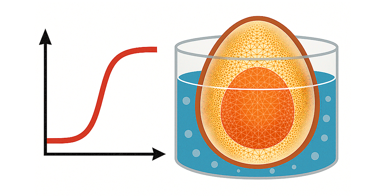
It’s time to answer the question on any breakfast-lover’s mind: “How long do I boil an egg?” While it seems so simple—place an egg in boiling water and wait—it would be remiss to say a fully hard-boiled egg is the only way to enjoy a delightful protein boost. We can use the finite element method (FEM) to simulate the conditions of an egg in water and find the ideal temperature and duration for the perfect egg by assessing temperature changes within the egg itself. We can then predict how long it takes to reach various consistencies, such as a runny yolk or a crumbly, fully set yolk.

Modeling complex physical systems often starts with breaking them down into manageable parts. That’s exactly what FEM does: it divides a complicated structure into smaller, simpler elements; solves the governing equations locally; and then assembles the results to capture the behavior of the whole system.

This approach makes it possible to simulate and analyze real-world scenarios without the cost and effort of physical prototypes. Here we’ll introduce the workflow of finite element analysis in Wolfram Language and walk through a simple example that covers the basics and highlights common issues that can come up along the way.

Our goal is to provide a general understanding of how to numerically solve partial differential equations (PDEs) using FEM, along with a practical resource you can use to build your own models.

Why Use Finite Elements?

Many PDEs (including classical equations like the Poisson or Schrödinger equations) don’t always have an analytical solution, especially if the region where we are trying to solve the equation is somewhat complicated. FEM is a valuable technique to solve PDEs numerically for at least two reasons: First, you can solve PDEs on arbitrarily shaped regions. Second, you can solve many types of differential equations, from the Laplace equation to Navier–Stokes equations.

Tools Needed for Finite Element Analysis

To solve a PDE with FEM, we need three things:

• A region that gets discretized into a mesh. This mesh consists of many small, simple subregions called elements. The key idea of FEM is to solve a simpler version of the PDE within each element and then combine these local solutions into a global solution that approximates the behavior of the original PDE over the entire region.
• The specific PDE we want to solve.
• Boundary conditions, which link the PDE to the world outside the region where the solution is being computed.

In Wolfram Language, FEM is implemented through the functions NDSolve, NDSolveValue and NDEigensystem, and we’ll be using NDSolveValue in our boiling egg scenario.

Engage with the code in this post by downloading the Wolfram Notebook

Version 1: Get a Workflow Started

We’ll build our model step by step, going through several versions and increasing the complexity of the model incrementally. We will start with a simple model, keeping in mind the sizes of objects and the units.

The first step is to define the geometry or region of the structure. Because an egg has axial symmetry, we will assume that analyzing a slice of the egg is adequate to describe its behavior. For FEM, we need to discretize the region into a mesh, and because a two-dimensional mesh does not need as many elements to approximate the geometry as a three-dimensional mesh would, our calculation will take less time. This is an important reason for using an axisymmetric model.

An average egg can be about 5 cm in diameter and 2.5 cm in radius. Because it is best practice to use SI units for the model parameters, we’ll define the egg radius as 0.025 m. At this point, we are purposefully ignoring any difference between the material of the yolk and the egg white. Our goal is to make this early version of the model as simple as possible.

Load the Finite Element package:

We’ll also set $HistoryLength to 0, which limits the number of previous results stored in the session to zero, saving computational memory at minimal cost.

Set $HistoryLength to 0:

Create a simple geometry of an egg:

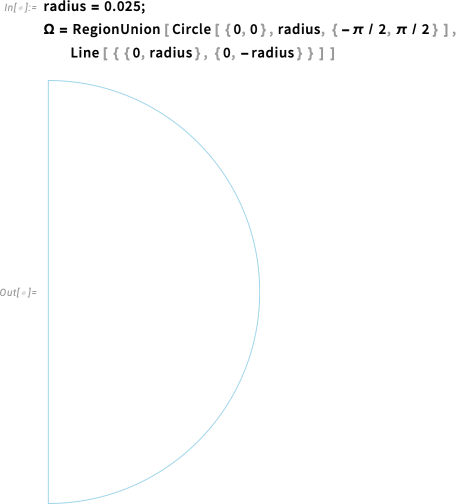
Also, we use ToElementMesh to generate a default finite element mesh from the geometry we’ve just created.

Generate the element mesh:

Visualize the finite element mesh:

To model PDEs in Wolfram Language, we use what are called PDE components, which are building blocks that help us specify the PDEs. These are functions that take in variables and parameters and return a PDE operator that can then be used with NDSolveValue. You can access the list of all the PDE components for any specific field. To study temperature evolution inside the egg, we’ll use HeatTransferPDEComponent to model the heat transfer over time.

The solution we are seeking, the dependent variable, is the temperature T (kelvin). For our cylindrical symmetry, we have two spatial independent variables: r is the radial coordinate (distance from the central axis) and z is the axial coordinate (distance along the axis of the cylinder). Both are expressed in meters. Because the boiling of an egg depends on time, we’ll also need the time variable t (seconds).

Set up the dependent and independent model variables:

We also need the parameters. For our first, simplified version, we’ll only specify the region symmetry as axis symmetric, and that will give us the correct terms for the egg slice we are focusing on. HeatTransferPDEComponent will fill the rest of the necessary parameters with default values, and that is fine for now.

Set up the parameters:

Next, set up the PDE operator. Here, op is the PDE operator—it’s just the left-hand side of the heat equation. So when we write op == 0, we’re really just writing the heat equation itself.

Set up the PDE operator:

Boundary Conditions

Initial and boundary conditions are important parts of PDE modeling because they contain information on the underlying physics of the process taking place. Boundary conditions specify the behavior of the solution on the boundaries. In this scenario, an important boundary condition is the outside of the egg, which is subject to the temperature of the surrounding boiling water. The initial condition is the starting temperature of the egg—whether the egg has been refrigerated or stored at room temperature.

Assuming the egg is at room temperature, we will use 20°C for our initial condition at time 0, then convert it to the SI base unit of kelvins.

Define the initial temperature in kelvins:

Set up an initial condition for the temperature inside the egg:

It is important to remember that boundary conditions and initial conditions must be consistent. One could be tempted to just set a temperature of 100°C to the outside of the region, representing the contact with the boiling water. While that is not entirely wrong, it has a problem. By our initial condition, all of the domain has an initial temperature of 20°C, even at the external boundary. Therefore, setting the outside boundary to 100°C contradicts that.

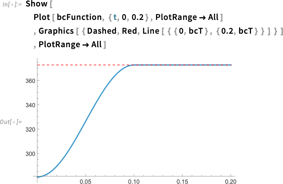
To avoid that in our scenario, we use a smooth step function that starts at the initial temperature and quickly gets up to the boiling temperature of 100°C. This is effectively modeling the act of putting the egg into the boiling water, which is a process on its own.

Specifically, we define the boundary condition using a piecewise function that equals 1 for times greater than one-tenth (1/10) of a second. For shorter times, it increases gradually, following a cosine function. Plotting the function makes this behavior clearer. This models the boundary temperature rising quickly—but smoothly—within the first 1/10 of a second after the egg is immersed in boiling water.

Specify the boundary temperature in kelvins:

Specify the temporal behavior of the boundary condition:

Visualize the temporal behavior of the boundary condition:

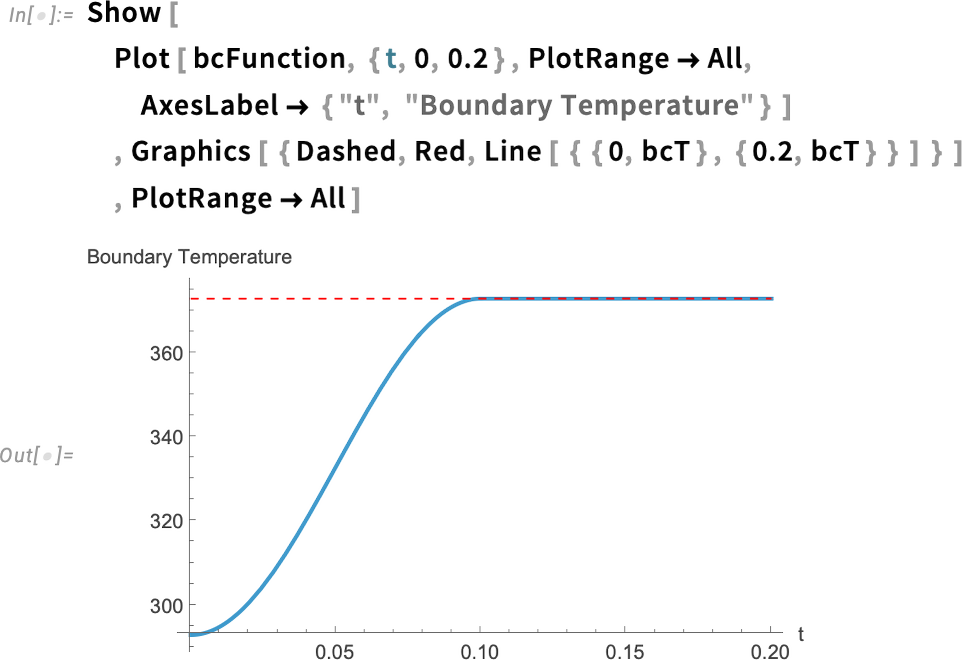
Now, we could simply define a DirichletCondition, which sets the value our dependent variable will have at the boundary:

But we will do something different that will be useful in subsequent versions of this model.

Visualize the point element marker:

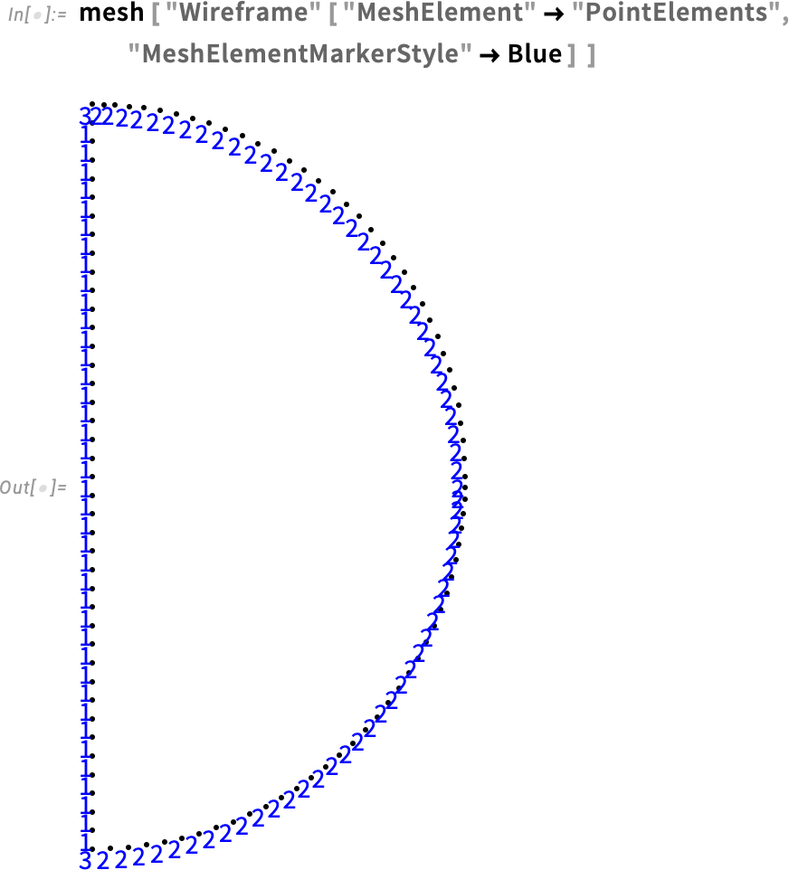
Our mesh visualization displays the point elements and element markers (see the Element Mesh Visualization tutorial for more information). We will take advantage of this to define the boundary condition.

With the help of HeatTemperatureCondition, we define a Dirichlet boundary condition. To specify the boundary, we take a look at the boundary element markers shown in our mesh. The boundary that will be in contact with water is labeled 2 and 3. Therefore, the boundary element markers are all but ElementMarkers == 1. So, we specify ElementMarkers != 1.

One advantage of using the function HeatTemperatureCondition is that it will take into account the parameters that we have defined.

Specify the boundary condition in kelvins:

Next, at the axis of symmetry, specify a symmetry boundary condition. We can do that with the HeatSymmetryValue function.

Specify the symmetry condition:

Notice that this evaluates to a Neumann zero value. If you need a refresher on Neumann values, check out these sources in the documentation:

• Solving Partial Differential Equations with Finite Elements
• NeumannValue

A Neumann zero value, in simple terms, indicates that the derivative of the temperature, taken normal to the axis of symmetry, is zero. Also, a Neumann zero value is the default if none is specified. Therefore, we will be omitting this for the following versions of this model. But it is useful to have that in mind.

Finally, we define how long the simulation time will be. As this is a simple first version, and we have used the default parameters for our PDE, we define a time of one second, which we will update later.

Define the simulation time:

To get our solution, we use NDSolveValue.

Compute the solution and store it in a variable:

Notice how it is specified. The operator op is our PDE defined earlier. Also, sym represents the symmetry condition, which we write as the right-hand side of the equation, but it is just a way of specifying the symmetry condition and Neumann values in general. Next in the list are the boundary condition and initial condition. I encourage you to look at the NDSolveValue documentation, which has many useful examples.

Inspect the solution:

We get an interpolating function that represents our solution, which we can later plot to visualize the solution.

Inspect the value for the solution at T = 0 at half the radius:

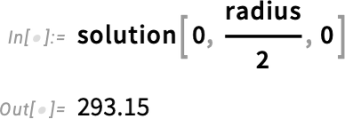
Call MinMax on the solution’s values:

Calling "ValuesOnGrid" gives the function values at each mesh coordinate. Then we can extract the minimal and maximal values from the solution.

To make this easier to interpret, let’s transform the temperatures to degrees Celsius, but the parameters going into the model will still need to be defined in kelvins. So let’s define an offset to convert between degrees Celsius and kelvin more easily.

Define an offset:

Then we can simply visualize the solution with a ContourPlot. Visualize the solution at half the simulation time:

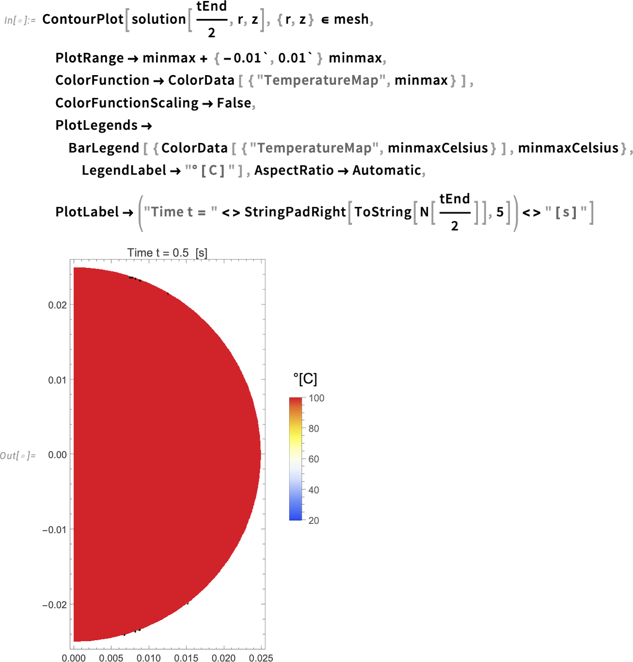
When we inspect the options for the ContourPlot function, we see that I use the minmax values in degrees kelvin for the PlotRange and ColorFunction, but I use the minmax values in degrees Celsius for the PlotLegends. This is to visualize the temperature in Celsius, which is easier to interpret than kelvin.

The plot seems to show that the whole region has a temperature of 100°C in just half the simulation time (0.5 seconds). To confirm that, let’s create an animation of the evolution of the temperature over time.

To save time later, we’ll go ahead and build a helper function for plotting.

Build a helper function to create contour plots of the temperature at various times:

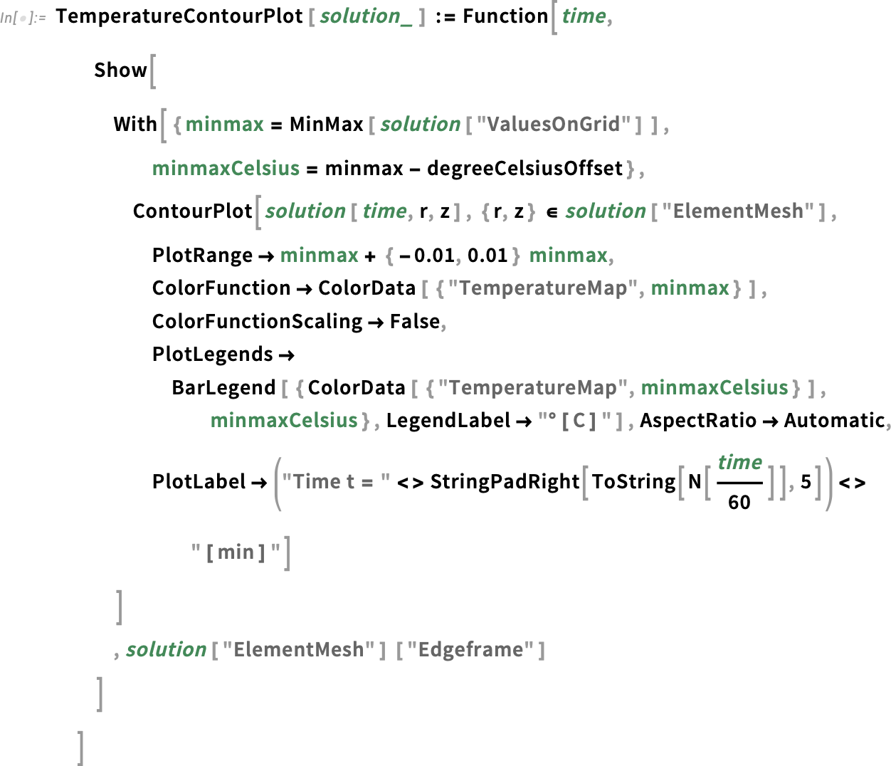
We get the "ValuesOnGrid" from the solution and take the minimum and maximum for our plot range. Show is used to display not only the solution but also the "Edgeframe" of the mesh. This is especially useful when we have subregions, as we’ll see later.

We have created a function of the variable time, which gives us the plot for a particular time. We then can map that function over a list of times.

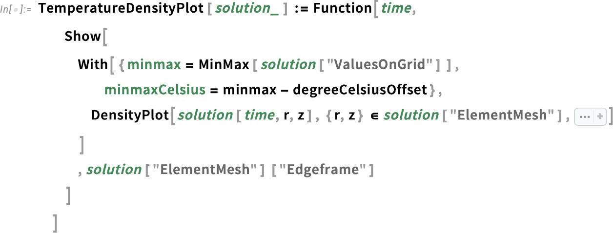
Some people prefer ContourPlot, but I like DensityPlot more. This is a similar definition following, but uses DensityPlot instead.

Define a DensityPlot version of the helper function:

Create a number of contour plot frames:

Rasterize the frames to make the notebook more lightweight (this is optional):

Animate the frames:

Here we choose a number of frames and divide the total simulation time into that number of frames, using Range to define a list of times. Then we map the helper function onto those times, resulting in a list of plots. Finally, we use ListAnimate to make an animation of all the frames.

The animation demonstrates that the entire region starts at the initial temperature and almost instantly heats up to 100°C (the temperature of the water), which doesn’t make much sense. But we didn’t expect this to be our final solution. For now, we know there are no errors or warnings in our simulation. This step was meant to get our workflow going—and that’s what really matters at this stage of the model.

Version 2: An Example of What Can Go Wrong

Now that our workflow is established, we start this next version by defining more realistic parameters instead of the ones that HeatTransferPDEComponent (the function used to generate the PDE) gives by default.

The heat equation includes three physical quantities that depend on the type of material we are modeling: density, heat capacity and thermal conductivity:

We will use estimates of the average values for both egg white and egg yolk to set the material parameters:

Inspect the parameters:

Set a realistic simulation end time of 10 minutes:

Regenerate the equations with the new parameters:

As we did before, solve the PDE:

So far, so good!

Let’s check the minimum and maximum values in the solution in degrees Celsius:

This is clearly wrong. A subzero temperature here doesn’t make any sense. Let’s plot the solution at the particular time it reaches that subzero temperature.

First, we must find the position in our region at which the minimum temperature value is located. By calling "ValuesOnGrid" on the solution, we can get all of the values of the solution, then use the Min and Position functions.

Find the position of the minimal value in the solution data:

By calling "Coordinates" on the solution and taking the first part, we get the time steps taken during the solution:

Find the time step at which the minimal value is stored:

In our badPosition variable, which is {{18, 386}}, the first number in the pair represents the index for the time at which our subzero value occurs. We can extract the problematic time by taking the eighteenth position in the time steps:

Now we can visualize the solution at that exact time.

Visualize the solution at the time step with the extreme values:

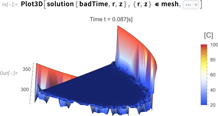
Here it is clear how early in the simulation there are a lot of oscillations near the boundary, and that’s the reason we are seeing extreme temperatures close to –2°C. The 3D plot displays overshoots and undershoots.

Let’s visualize that better with the element mesh. To do that, we make a projection of our 2D mesh into 3D with ElementMeshProjection. We use Show to display both the 3D plot for our solution at the problematic time and the element mesh.

Zoom in to the solution plot and visualize the underlying finite element mesh:

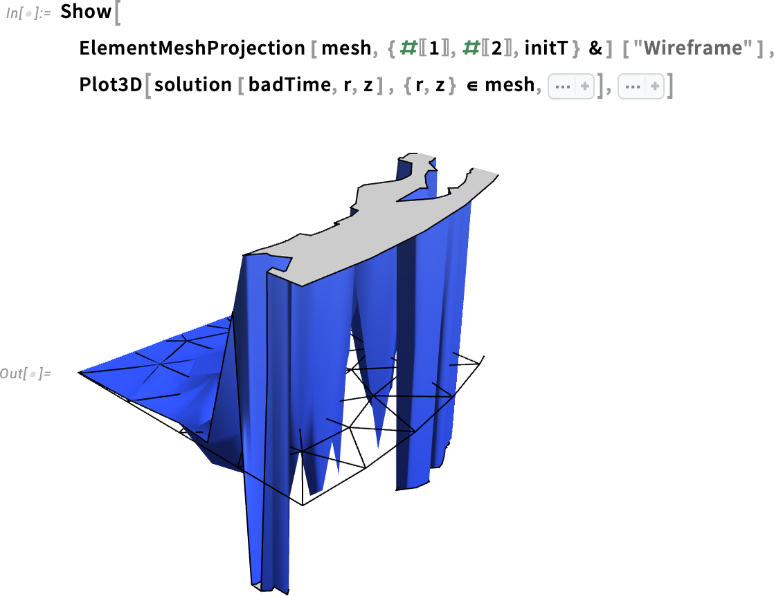
I encourage you to review the documentation for ElementMeshProjection to learn more about how to visualize a 2D mesh as 3D.

It is now clear that the undershoots are happening within a few elements from the boundary. But what could be causing these over- and undershoots?

Let’s find the minimal length of the elements in our mesh. We take the average area of the elements and, by using Sqrt, we get a number related to the edge length of each element. Then we take the minimum of that.

Get the minimal edge length of the mesh in meters:

The distance between elements is about 1 mm, which means that the first elements near the boundary have an edge length of about 1 mm. On the other hand, given that our initial temperature is 20°C and our boundary temperature is 100°C, the change in temperature between the boundary and the rest of the region is about 80°C.

Trying to resolve that abrupt change of about 80°C at the boundary with elements of that size is not sufficient. That is likely the reason we are getting temperatures that are far below the initial temperature, where there are not any heat sinks. Therefore, the mesh needs to be refined.

If we refine the whole mesh, it probably will solve our problem, but the refinement is not needed in the center of the egg. Refining the whole mesh now will slow the simulation, so it’s best to refine the mesh just near the boundary (the eggshell).

We will create a signed distance function first and, from that, use MeshRefinementFunction to redefine our mesh.

SignedRegionDistance gives us the distance to the boundary of a region from a specific point. It gives a negative value when we are inside the region and a positive value when we are outside it. In our case, we can define that for a Disk with the same radius as our “circular” egg.

Create a signed distance function of the whole egg region:

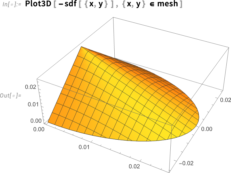
We can visualize the signed distance function and see how it decreases linearly as it reaches the boundary. This outcome makes sense, because the distance at the shell to the shell is predictably zero.

Visualize the refinement function over the meshed geometry:

Next, we create our refinement function, which takes the vertices of the mesh and its area and returns either True or False. If the output is True, a refinement will take place there; if False, it will do nothing.

Create the mesh refinement function:

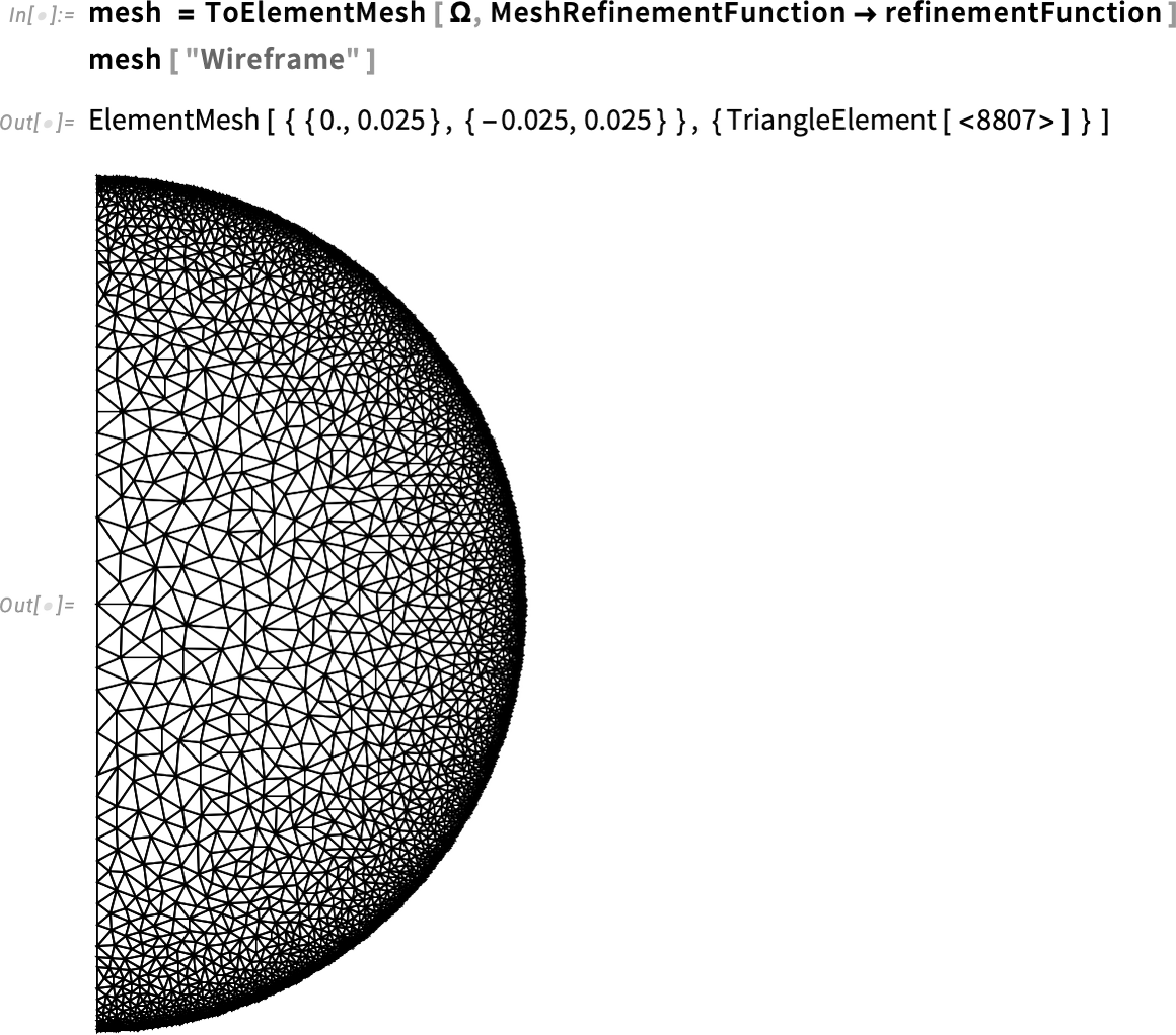
Then we set the MeshRefinementFunction option inside ToElementMesh to our refinementFunction.

Redefine the mesh:

Next, we will use NDSolveValue to obtain the solution, but now we wrap the calling of the function with Monitor, which will help us inspect the time steps by printing the time variable during the computation. This will give us an idea of how long it will take to finish the whole computation. Monitor is used outside the call to NDSolveValue, and the EvaluationMonitor option is used inside NDSolveValue. This is particularly important when we refine the mesh, because it may take longer because of the refinement.

Solve the PDE and monitor the progress:

Inspect the temperature range of the newly found solution:

Great! Now we get a temperature range that we would expect. There will be, of course, a bit of numerical error intrinsic to the method—that is, the range will not be {20, 100} exactly. But this is promising.

We can proceed to create our animation as usual by calling the helper function we defined with our new solution, rasterizing the frames and then animating them.

Create the frames for the solution:

Rasterize the frames:

Animate the frames:

We can see that the over- and undershoots problem is solved. This demonstrates how important it is to check that our solutions make sense and how we can modify the mesh as needed.

At this point, we get a good idea of how the temperature spreads in the boiling of the egg. Let’s calculate the temperature at the center of the egg after six minutes of cooking.

Inspect the egg’s temperature at r = 0 and z = 0 after six minutes:

The result is 41.6°C. This value likely doesn’t represent the actual temperature of the egg yolk in a real egg, because we are currently making too many assumptions. However, it is a good reference for now.

In this version, we used a basic model that disregarded the existence of two different regions—the egg yolk and egg white. We will address that in the next version.

Version 3: Represent Multiple Material Regions

In this version, we will consider two different regions by first defining the innerRadius, which is half of the outer radius. Then we can define two half-circles and use RegionUnion to create a single geometry.

Create a multi-material geometry:

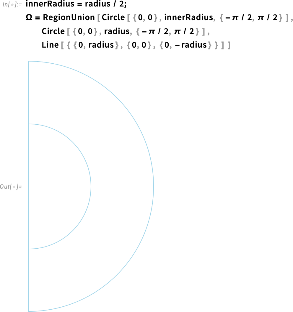
Here we define material region markers in order to differentiate the parameters for the two regions later. This will make our code clearer, as we’ll see.

Specify material region markers:

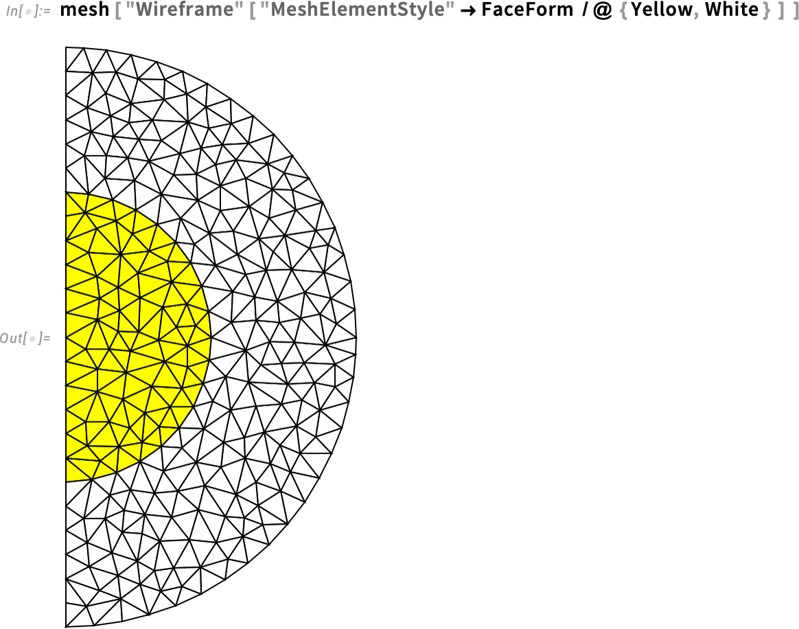
We use the "RegionMarker" option to distinguish the two regions by assigning a different marker to each subregion. The option is given as a list of lists, where each inner list contains a point within the subregion and its associated region marker.

Create a mesh with material markers:

We can visualize it with different colors, by specifying "MeshElementStyle" in the "Wireframe" options.

Visualize the multi-material mesh:

Visualize the point element markers:

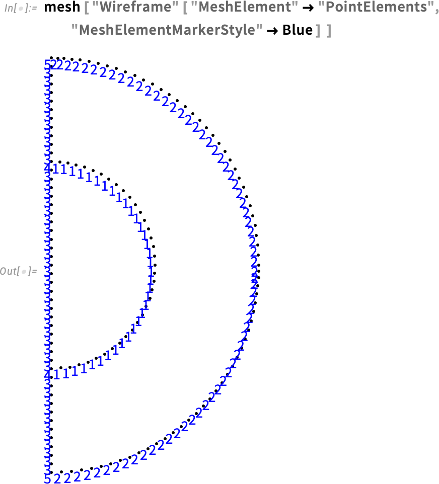
Since we changed the region, the element markers for the boundary also have changed. Therefore, we can redefine the boundary condition for markers 2 and 5.

Keep in mind that these are element markers for the boundary. They are different from the region markers we defined earlier. Don’t confuse the two.

Regenerate the boundary condition:

After visualizing the point element markers, we redefine the mesh by specifying the mesh refinement function as before.

Create a mesh with material markers and a mesh refinement:

Visualize the refined multi-material mesh:

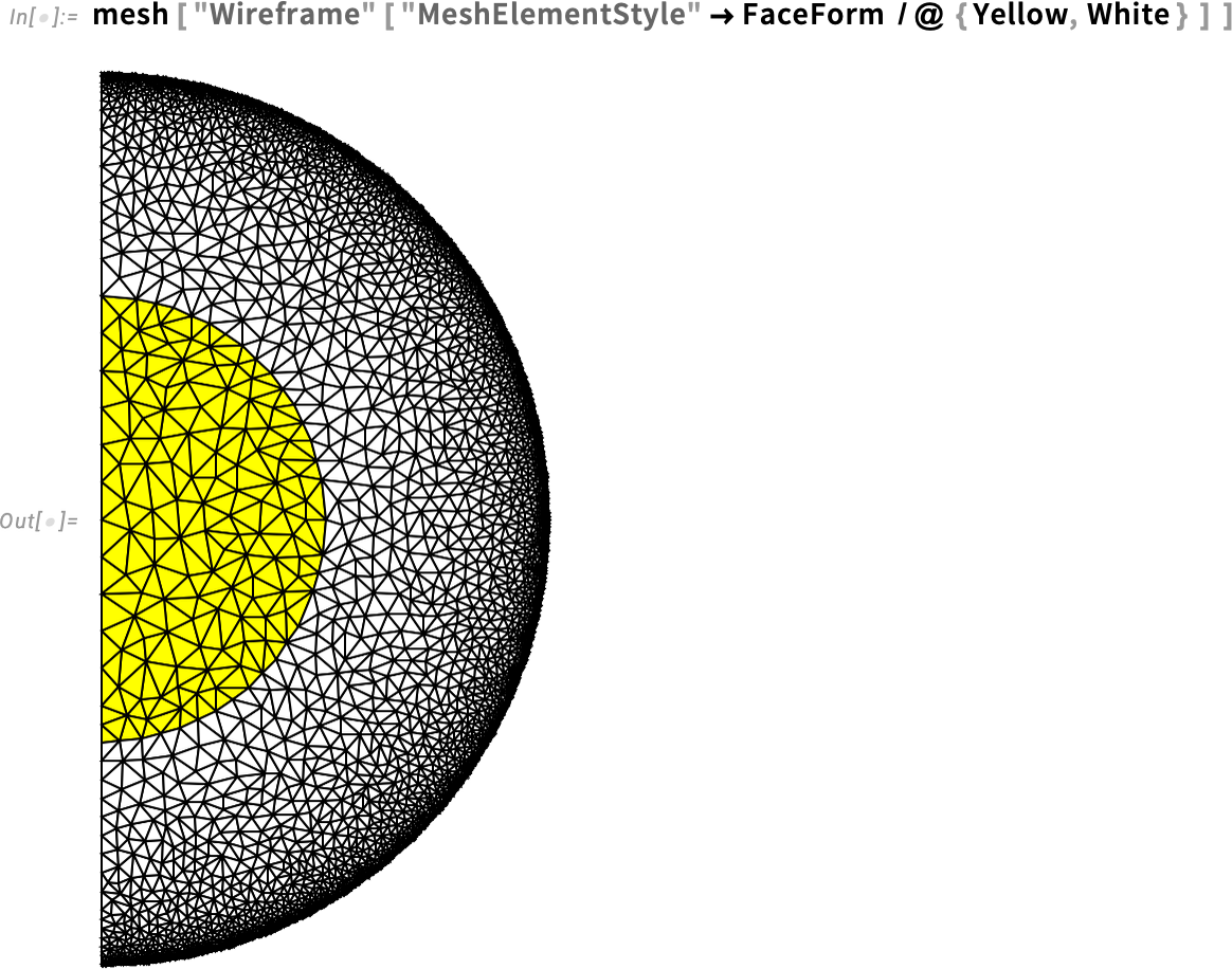
Great result! But before solving the problem, we will redefine the parameters for each material, using estimates of the average values for mass density, thermal conductivity and heat capacity for egg yolks and egg whites based on the findings of “Density, Heat Capacity and Thermal Conductivity of Liquid Egg Products.”

To specify the material parameters, we use the Piecewise function for each physical quantity:

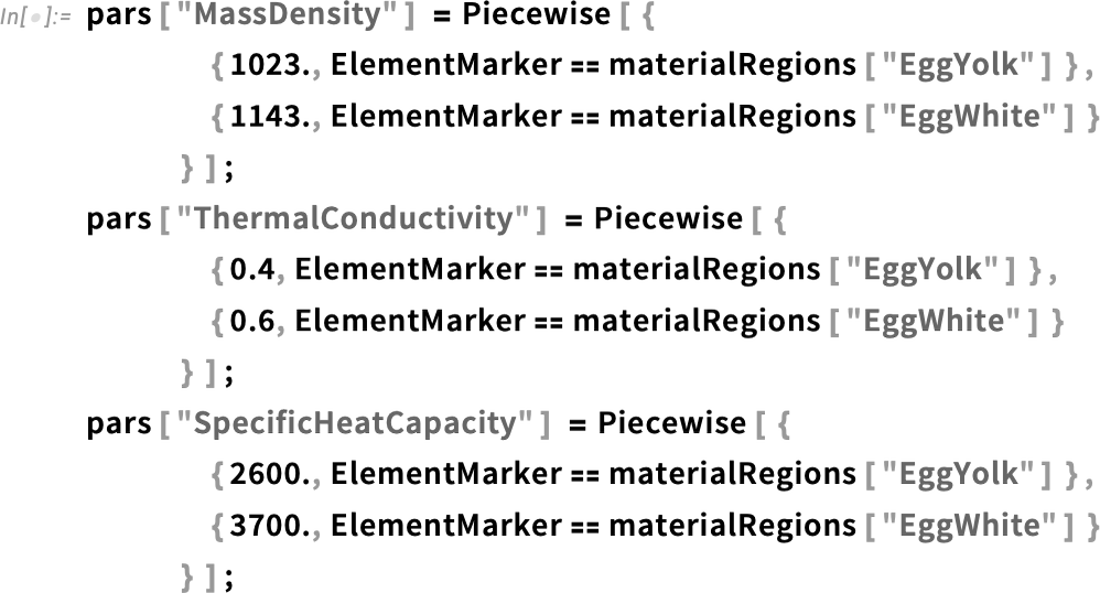
Then we can regenerate and solve the PDE as we did before.

Regenerate the partial differential equation:

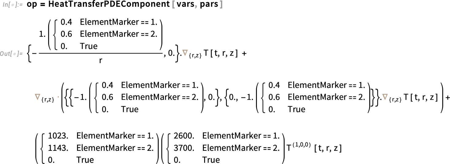
Solve the PDE:

Inspect the temperature range of the new solution:

The resulting temperature range is reasonable. Let’s visualize the solution.

Create the frames for the solution:

Rasterize the frames:

Animate the frames:

Here we see even heating of the egg, similar to our last version with only a single region. However, this version is more accurate because we have a better model of the real structure of the egg.

Inspect the egg’s temperature at r = 0 and z = 0 after six minutes:

In this solution, the temperature result of 38°C again seems too low for the given time. In fact, this temperature is even lower than the previous result of about 42°C.

We need a way to know which parts of the egg are cooked after a given time.

Version 4: Refine the Model Further

In this version, we will refine the data used for the physical quantities involved in the model. We will also predict whether the egg is cooked by comparing the results with the denaturation temperatures of the egg yolk and egg white (i.e. the temperatures at which egg proteins begin to unfold and solidify).

To refine the physical quantities (density, heat capacity and thermal conductivity), we will rely on the data provided by these two studies:

• Coimbra et al., “Density, Heat Capacity and Thermal Conductivity of Liquid Egg Products,” Journal of Food Engineering, 2006
• Abbasnezhad et al., “Thermophysical and Rheological Properties of Liquid Egg White and Yolk During Thermal Pasteurization of Intact Eggs,” Journal of Food Measurement and Characterization, 2025

In the previous version, we had good estimates of the physical quantities for both the egg yolk and egg white. But in reality, those quantities may change over time as the egg heats up. A better model is one that takes into account how these quantities vary with temperature.

Using data from the studies mentioned previously, we will set up pairs of temperatures and the corresponding physical quantity (in SI base units). Our goal is to model each physical quantity (density, thermal conductivity, heat capacity) as a function of temperature.

Let’s start with density. Notice that there is a density data definition for both the egg yolk and egg white.

Set up measurement data for the mass density of the egg yolk and egg white:

With that, we can create two interpolating functions, one for the yolk and one for the white, using Interpolation.

Create an InterpolatingFunction for the mass density data:

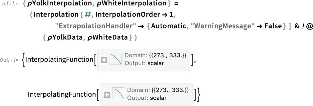
The "ExtrapolationHandler" option is used to handle points that fall outside the range of our available data. Our data is not perfect and does not cover the entire range of temperatures. Since properties like density vary almost linearly, extrapolating from the existing data provides a reasonably accurate approximation.

Visualize the measured data and the interpolated functions:

We can see how the density decreases as temperature increases. Although we don’t have temperature data beyond 335 kelvins, we do have a reasonable extrapolation from the data.

Now we repeat the same process for conductivity.

Set up measurement data for the thermal conductivity of the egg yolk and egg white:

Create an InterpolatingFunction for the thermal conductivity data:

Visualize the measured data and the interpolated functions:

We can see how conductivity increases slightly with temperature, and, again, we have a reasonable extrapolation of the data.

For the specific heat capacity, we have a slightly different approach. We have fewer data points, and the quality of the points is not as good as for the other two quantities. The optimal approach is to do a linear fit of the data, which will give us a linear function that best fits the data.

Set up measurement data for the heat capacity of the egg yolk and egg white:

Create a LinearModelFit for the heat capacity data:

To explore how the function works in more detail, refer to the LinearModelFit documentation.

Visualize the measured data and the linear function that fits it:

The plot displays a reasonable approximation of the data and a good extrapolation at higher temperatures.

Now that we have the functions for the physical quantities, we only need to specify them as piecewise functions, as we did before:

Regenerate the partial differential equation:

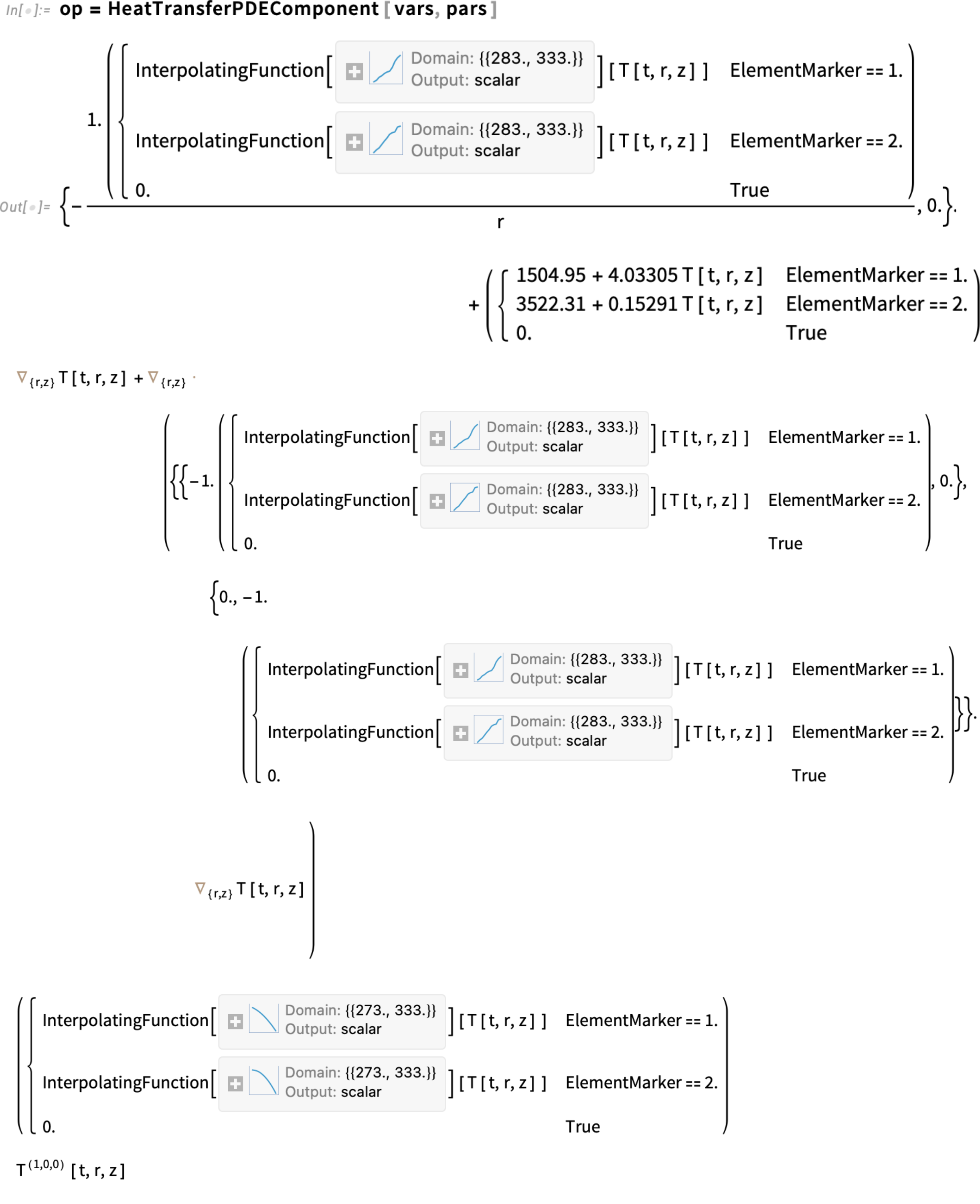
An important consideration: mass density, thermal conductivity and heat capacity are now functions of temperature T. At the same time, T is the dependent variable for which a solution is sought. This mutual dependence means the coefficients in the equation vary with the solution itself, making the PDE nonlinear. Nonlinear models typically require more time and computational effort to solve. That’s why it’s often a good idea to start with an unrefined mesh while setting everything up. Once you get a reasonable solution, you can switch to a refined mesh for better accuracy. However, in this case, we’ll go ahead and use the refined mesh.

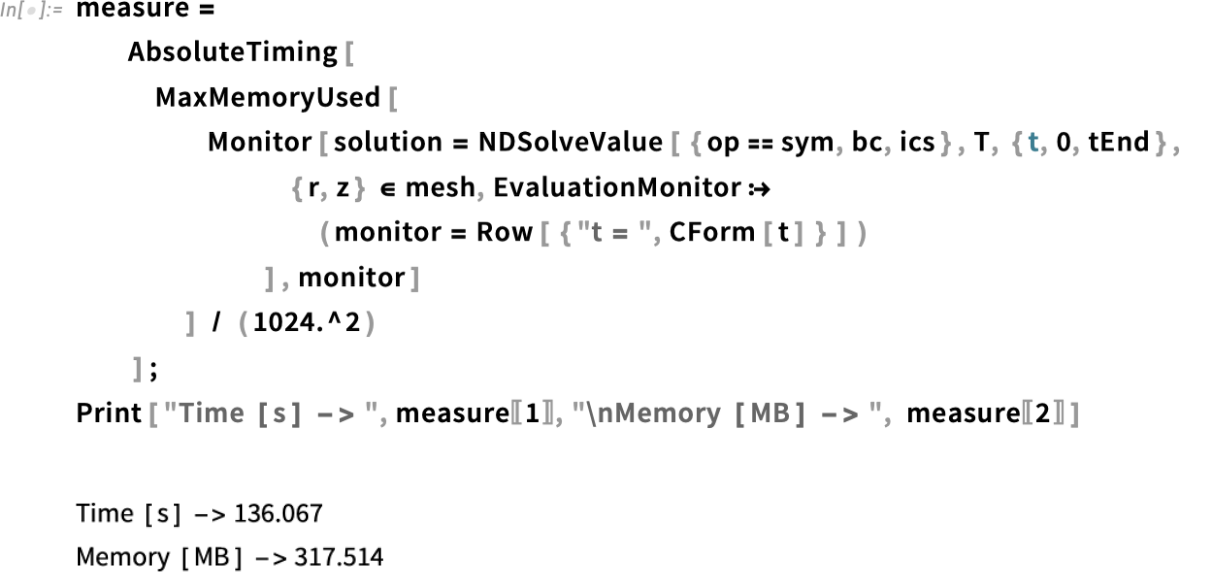
Since we haven’t changed the geometry or the boundary conditions, and we have only redefined our PDE operator with the new parameters, we can go ahead and solve the PDE. Here we use AbsoluteTiming to get the time spent on the entire calculation and MaxMemoryUsed to see how much computer memory it consumed.

Now we solve the PDE, monitor the progress and measure the computational time and memory it takes (around three minutes on a normal laptop).

Solve the PDE:

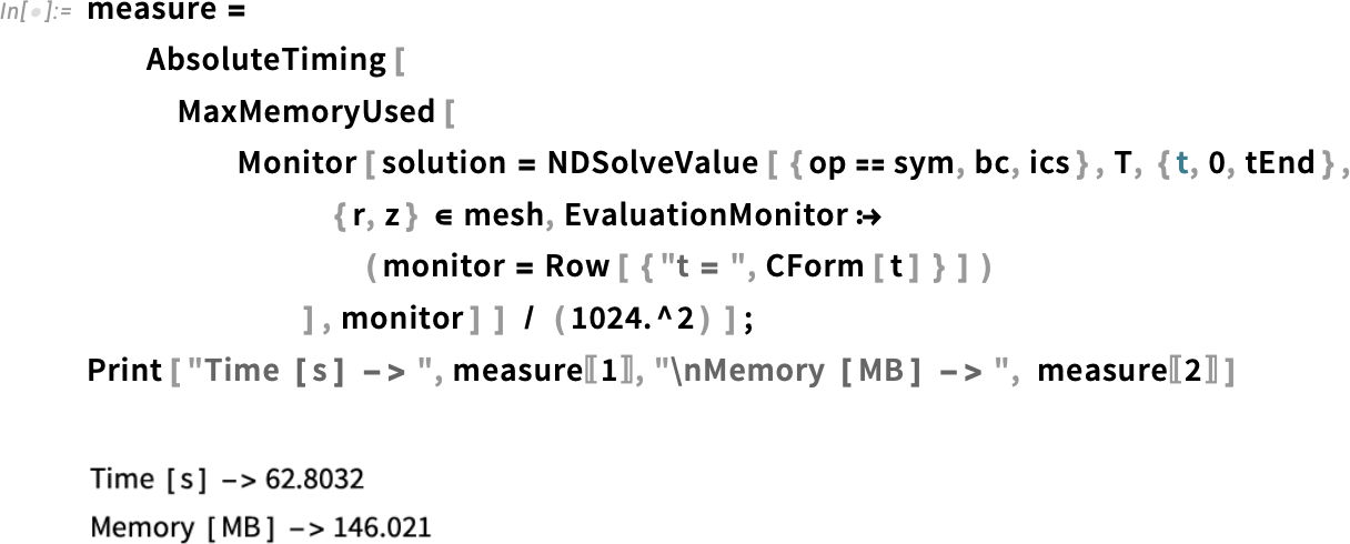
This increase in computation time is expected for most nonlinear models.

Inspect the temperature range of the newly found solution:

Before visualizing our solution, we will define the denaturation temperatures of the egg yolk and egg white. This will give us a good idea of whether the two regions of the egg are cooked at a certain point in time. These temperatures are from the Journal of Food Measurement and Characterization study cited earlier.

Set the denaturation temperature for the egg white:

Set the denaturation temperature for the egg yolk:

We can visualize the denaturation temperatures along with the animation of our solution. The best way to do that is a contour plot with a contour line that indicates the point in the region with the denaturation temperature.

I prefer the density plot, so here we define a new function called TemperatureDenatureDensityPlot, which calls the previously defined helper function TemperatureDensityPlot. We are using Show to display the plot as before, but with the contours for the denaturation temperatures of the egg yolk and egg white. The contours are plotted with an additional ContourPlot.

Build a helper function to create a density plot of the temperature distribution and visualize the denaturation temperatures:

Create the frames for the solution:

Rasterize the frames:

Animate the frames:

The denaturation temperature for the egg white is shown with the green dashed line, and the denaturation temperature for the egg yolk is shown with the magenta dashed line. The plot shows the diffusion of heat inside the egg, as we would expect.

At the six-minute mark, we can see that the whole egg white has surpassed its denaturation temperature. This is a promising result for our model.

However, if we look at the 10-minute mark, the whole region surpasses the egg white’s denaturation temperature, while part of the egg yolk has not surpassed the yolk’s denaturation temperature, which indicates the yolk is not sufficiently cooked, even at 10 minutes.

Hard-boiled eggs generally cook for 10–12 minutes, so 10 minutes should result in a fully set egg yolk. Therefore, our model is not complete yet, since it indicates that after 10 minutes the egg yolk is not fully cooked.

Inspect the egg’s temperature at r = 0 and z = 0 after six minutes:

Inspect the denaturation temperature of the yolk:

In versions 2 and 3 of the model, we got temperatures of 38°C and 42°C, respectively. Here in version 4, we get about 40°C for the temperature at the center of the egg at the six-minute mark. Compared with the denaturation temperature of the yolk, this still seems too low. We need to improve that in the next version.

Version 5: Build a Realistic Egg Geometry

When the model is not giving us the answer we’re expecting, it can be a good idea to refine it further. One way of doing this is to take a look at the assumptions we have made. One important assumption is that the egg has a circular shape, which, of course, is not true in reality. In this version, we will create a more realistic geometry for the egg.

We can still assume that the geometry of the egg yolk is well modeled by a circle. But we can approximate the geometry for the eggshell in a more realistic fashion.

To do that, we’ll use a mathematical equation that approximates the geometry of the eggshell, based on this reference.

Create a helper function to compute the coordinates of the shape of an egg geometry:

This new function uses Table to create a list of pairs (or points) that define the eggshell. The equation that models the shape of the eggshell accepts three parameters: the length of the egg (from base to top), the breadth or width of the egg and a parameter that controls the elongated appearance of the egg.

Manipulate the parameters to view different shapes:

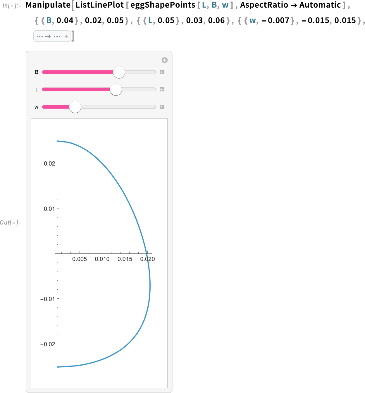
Inspect the value of the radius:

We will call the new eggShapePoints function for an egg that is 5 cm tall and 4 cm wide.

Create coordinates for the egg geometry by specifying parameters:

Using the coordinates that define the eggshell, we construct a B-spline curve—that is, a piecewise polynomial curve that best approximates the points outlining the eggshell. We simply pass the coordinates to the BSplineCurve function, and it returns the spline curve that defines the eggshell.

Create a spline:

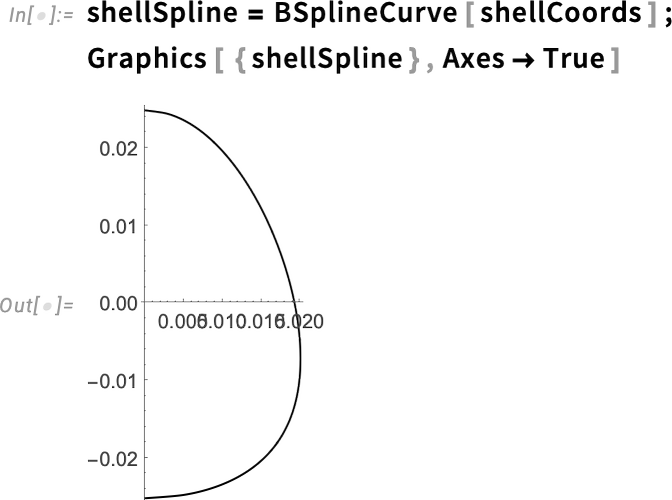
Then we can use RegionUnion, joining a half-circle with our eggshell curve, to create the skeleton of our region. This is just as we did earlier, but with the spline curve for the eggshell.

Create an egg geometry with a subregion:

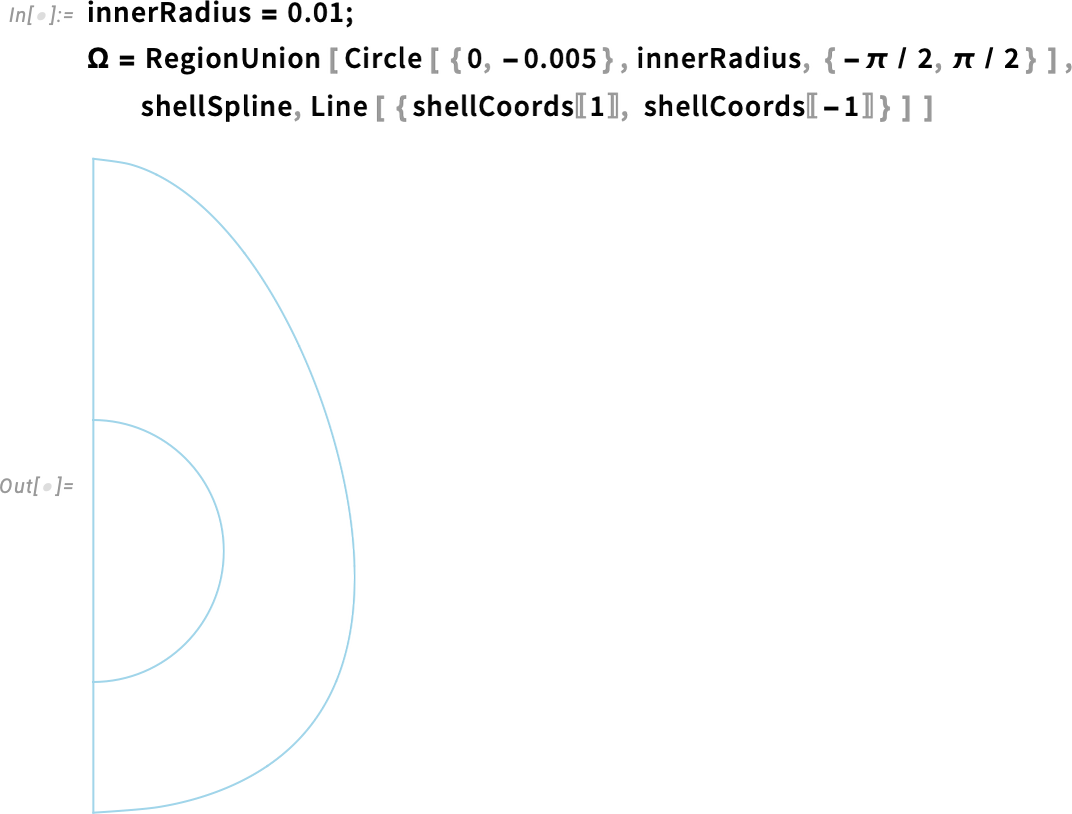
Next, we create the mesh with the region markers, as we did earlier.

Create a mesh with material markers:

Visualize the point element marker:

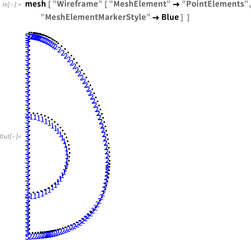
As we can see, the markers for the outside of the egg are still 2 and 5, so we don’t need to redefine the boundary condition.

Inspect the boundary condition:

Inspect the refinementFunction:

We are at a good point already, but we have a slight problem. For our previous version, we created a refinement function based on the region having a circular shape. We need to create a new refinement function for our new region:

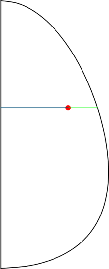
We can refine the elements based on their radial distance to the shell, which is shown as a green line in the image. The red point represents an element, and it has a radial distance to the axis of symmetry (the blue line) and a radial distance to the shell.

We want to define a refinement function based on the distance in green. The higher the distance to the shell, the lower the refinement; the lower the distance to the shell, the higher the refinement. Furthermore, to get the green line distance, we subtract the blue line distance from the distance from the axis of symmetry to the eggshell (shown in magenta):

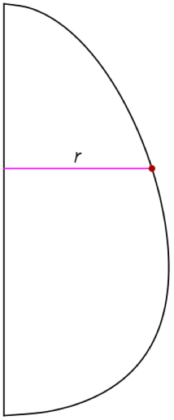
First, we define a function that returns the value of the cylindrical coordinate r for a given z in the eggshell curve.

Do an interpolation of the shell’s coordinates:

We are simply flipping the order of the points in the shell coordinates—replacing {r, z} with {z, r}—and then doing an interpolation from that. Here, rShell is an interpolating function that takes z and returns r.

Plot the function that gives the rShell function:

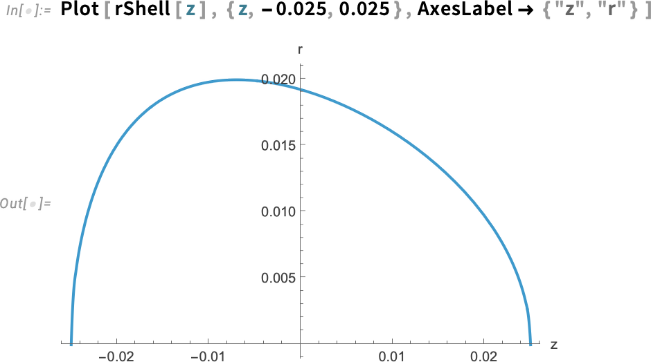
The plot of this function is what we would expect: the coordinate r for the eggshell as a function of z.

Then the only other thing we need to do is compute the distance from the axis to the shell minus the absolute value of the coordinate r for each point. This will give us the distance from each point to the shell (shown in green):

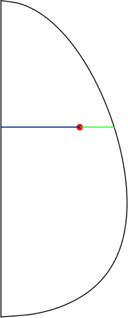
Define a function for the radial distance to the shell and plot it:

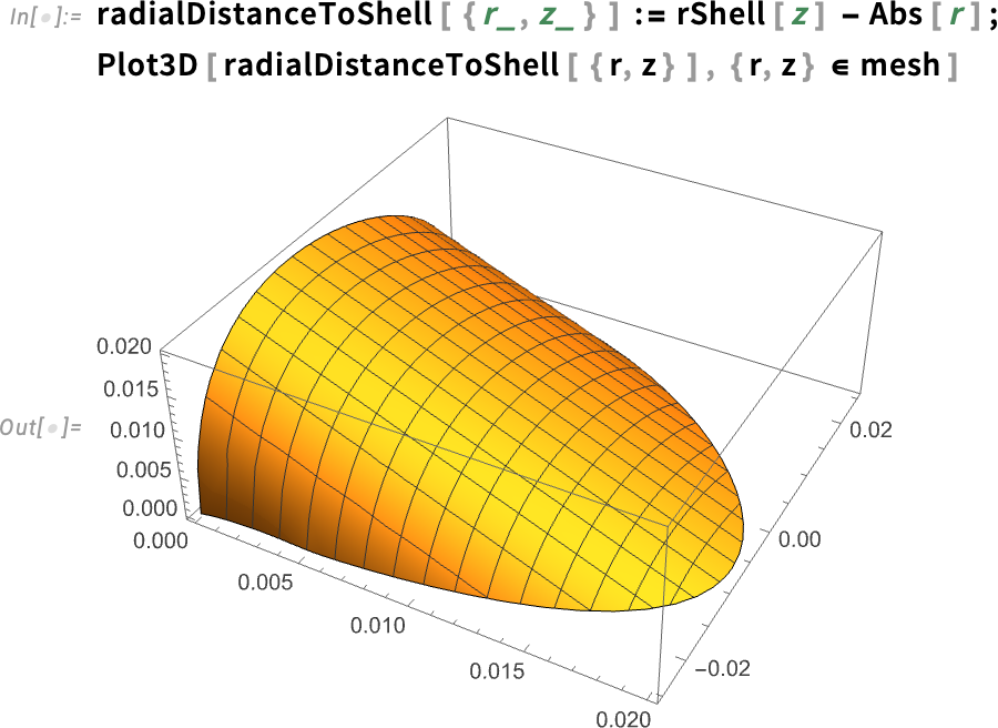
The plot shows that the distance from each point to the shell decreases almost linearly, as we would expect.

Plot the distance to the shell cubed:

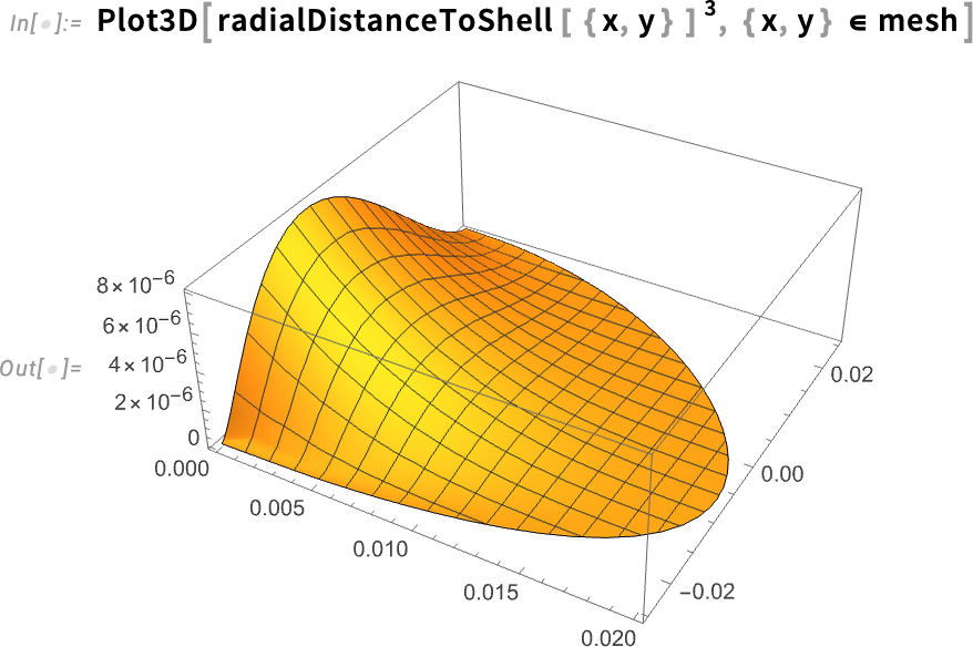
When we plot the distance cubed, the values decrease more quickly as the distance to the shell becomes smaller.

Keep in mind that finding the correct behavior for the refinement function is a trial-and-error process.

Define the refinement function:

Here we defined the refinementFunction such that an element gets refined if its area is greater than the distance to the shell cubed, with some offset to avoid refining too much. In other words, the size of the elements are proportional to the distance to the shell cubed. The closer to the shell, the smaller the elements.

Define the mesh using the MeshRefinementFunction option:

Visualize the multi-material mesh:

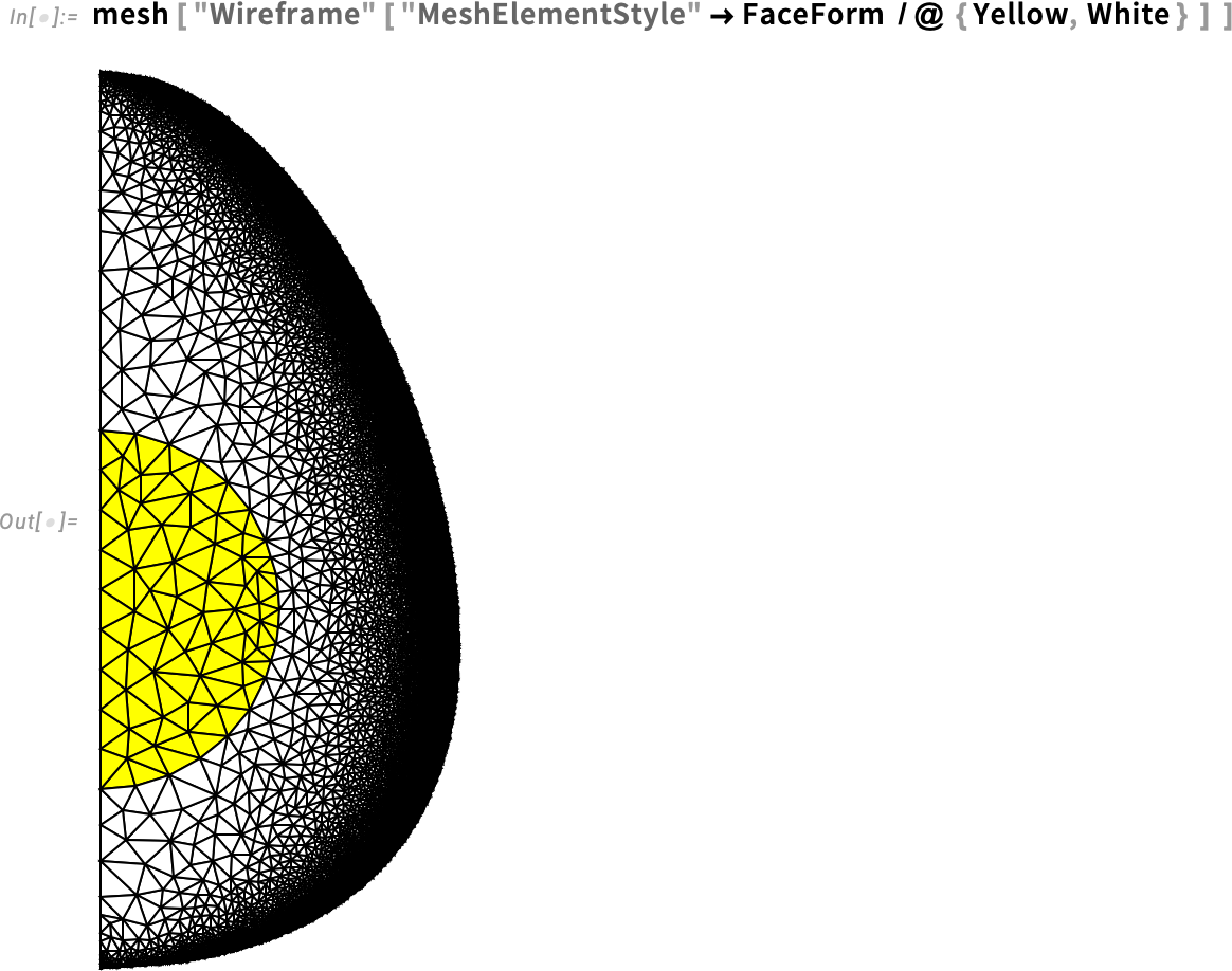
As we can see, the elements near the center of the egg are not refined at all, but we get a very fine refinement near the eggshell.

We can proceed to solve the PDE as before, measuring the time and memory expended. This calculation of a nonlinear model with this mesh takes about six minutes to finish (just like the eggs I like to eat!). Keep computing time in mind when developing your own models. This is why Monitor is useful, and why using a non-refined mesh at first is a good idea.

Solve the PDE, monitor the progress and measure the computational time and memory it takes:

Inspect the temperature range of the newly found solution:

Again, we get a reasonable range of temperatures, so we can proceed with the animation.

Create the frames for the solution:

Rasterize the frames:

Animate the frames:

Two important points: First, at six minutes, the egg yolk is still not cooked, which is something we expected. Second, at 10 minutes, the whole region has surpassed the denaturation temperatures for both the egg white and yolk, so we can assume that the egg is fully cooked at this point. The model now reflects a realistic time frame to cook the egg. Great!

Inspect the egg’s temperature at r = 0 and z = 0 after six minutes:

At six minutes, we have a much more realistic temperature of nearly 60°C in the center of the egg, compared with our previous version of the model, in which the center only reached about 40°C. We can conclude that geometry plays a crucial role in the dynamics of heating the egg.

Version 6: Use the Model

Now that our model is producing satisfactory results, we can use it to make predictions.

Previously, our egg was introduced to boiling water from room temperature. Let’s now model a more realistic case in which the egg is taken straight from the refrigerator, where we’ll be assuming that the egg has an initial temperature of 8°C. To model that, we have to modify our initial and boundary conditions. In particular, the boundary condition needs to start from our new initial temperature and quickly rise to 100°C.

First, we set the initial temperature to 8°C and convert it to kelvins.

Set the initial temperature of the egg:

Next, we define our new initial condition.

Set an initial condition for the temperature inside the egg:

It is also necessary to modify the boundary condition function, which now starts from the new initial temperature.

Specify the temporal behavior of the boundary condition:

Visualize the temporal behavior of the boundary condition:

Regenerate the boundary condition:

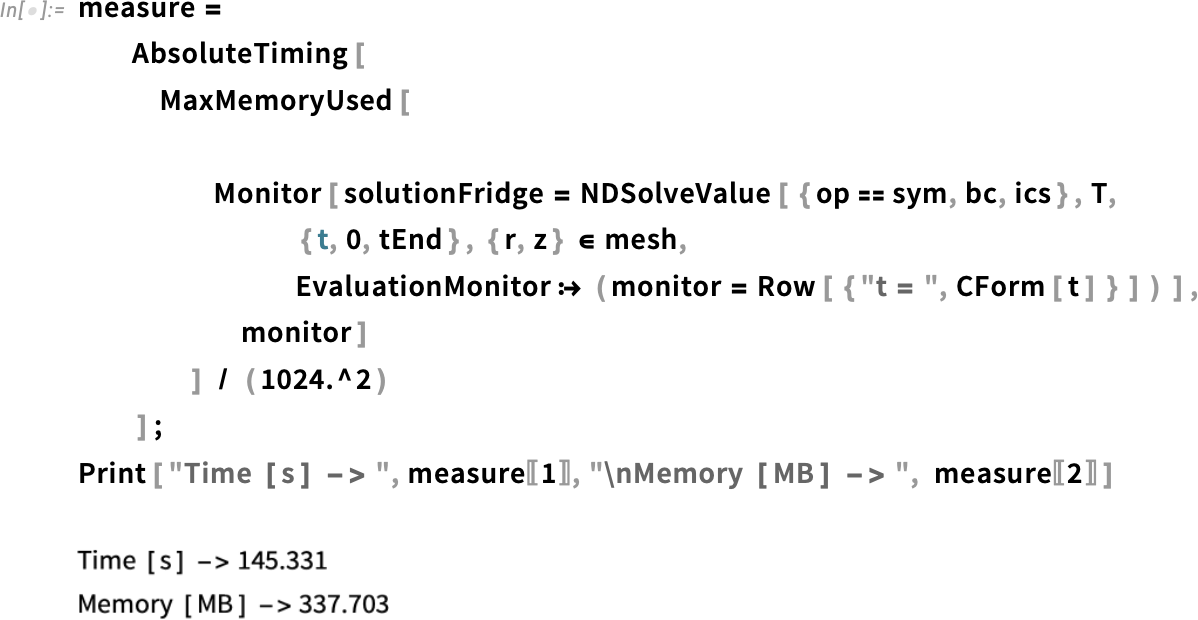
Then we solve the PDE as before. Note that here we store our solution in a new variable called solutionFridge, so that we can compare it with our old solution.

Solve the PDE, monitor the progress and measure the computational time and memory it takes:

Inspect the temperature range of the newly found solution:

We get a range that’s reasonable for our refrigerated egg.

We can plot the solution in the same way as before.

Create the frames for the solution:

Rasterize the frames:

Animate the frames:

At six minutes, the egg yolk is still not cooked, just as in our last version. At 10 minutes, the egg seems to be cooked all the way through. It is difficult to see just by looking at the animation if there are any meaningful differences between the refrigerated egg and the room-temperature one.

One good option is to plot the temperature for the line that passes through the center of the yolk to the eggshell for both solutions—the refrigerated egg and the room-temperature one. A simpler plot might reveal more subtle aspects that are difficult to see in the density plot.

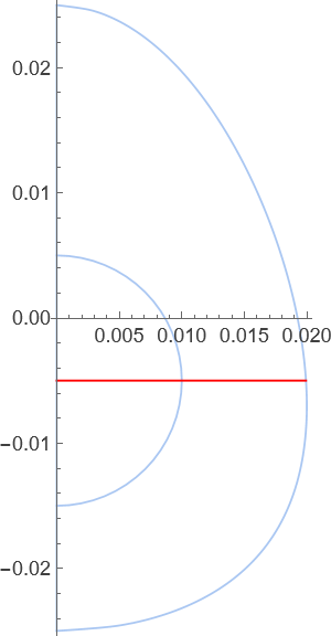
We are plotting the temperature for the values of r that lie on this line. We need the value of r for the right boundary. With our function rShell that we defined earlier, we can get the value of the coordinate r for the z value of 0.005, which is the center of the egg yolk.

Get value of r for the line:

Now we know the value of r for the right boundary of the line we are interested in. Next, we want to know how the temperature increases for that line, specifically for the values of r between 0. and 0.0179. We can create a simple plot, at six minutes for example, for those values of r.

Plot the solution along the radial line from the center of the yolk to the exterior of the egg at six minutes:

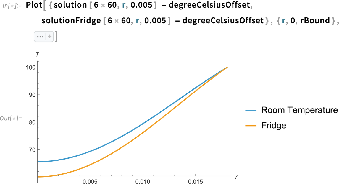
We can see that the temperature at six minutes is lower for the egg taken straight from the fridge compared to the room-temperature egg for all the values of r. In particular, we can see a difference of about 5°C at the center of the egg.

Because we are interested in predicting whether the egg is cooked, we also need a way to visualize the denaturation temperature. One way to do this is by plotting a vertical line that marks the value of r at which the egg reaches the denaturation temperature.

We can use FindRoot to find the value of r that makes the solution equal to the denaturation temperature.

Get the value of r at which the solution is equal to the denaturation temperature:

We find that the denaturation temperature for the yolk of the egg taken from the refrigerator is reached at a radius of about 10 mm (1 cm) from the center. We can represent that with a line in our plot.

Plot the solution along the radial line from the center of the yolk to the exterior of the egg:

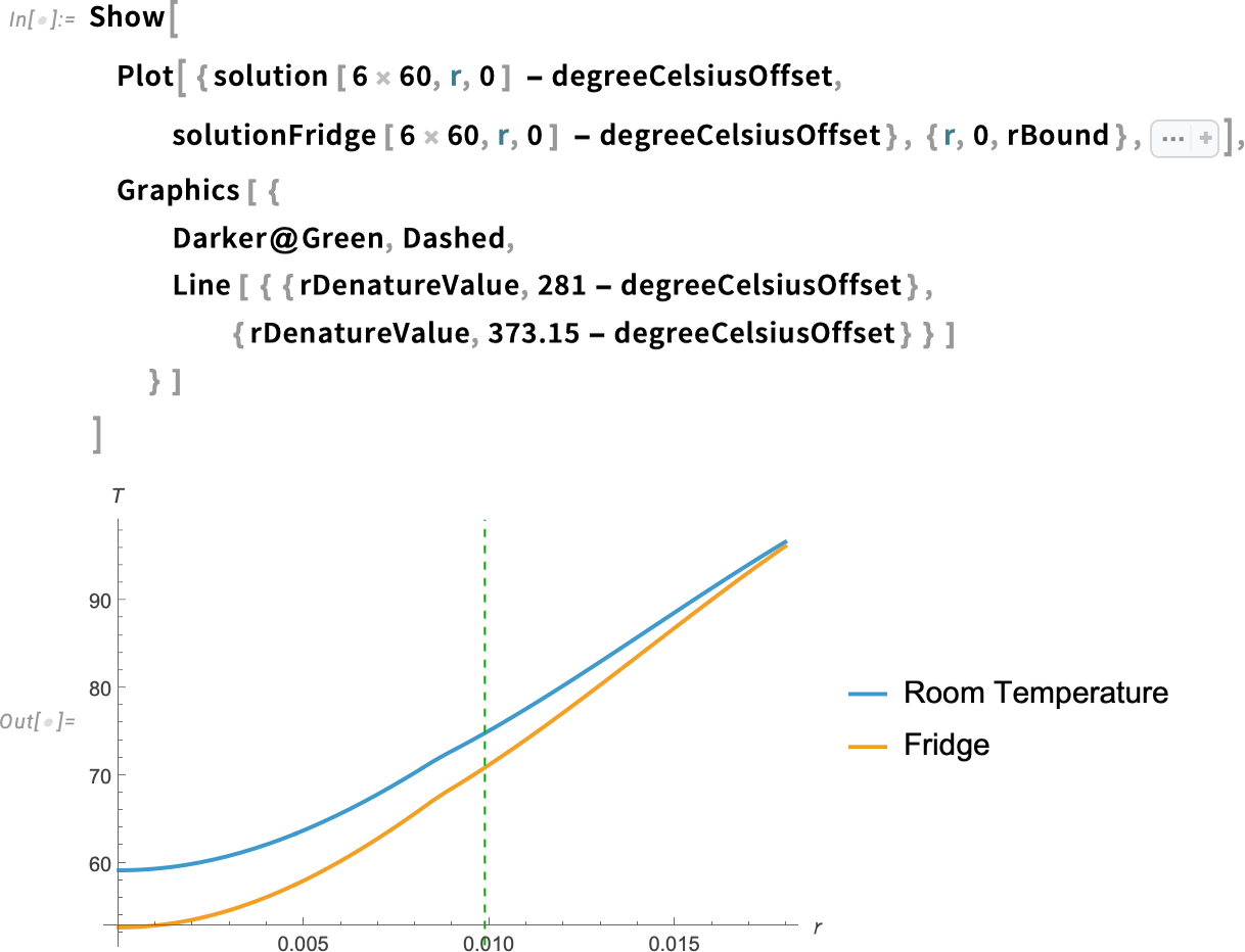
In addition to the egg yolk, we also need the egg white denaturation temperature for both the room-temperature egg and the refrigerated egg. Instead of doing this manually, we can define a helper function.

This function takes the solution and the value of the denaturation temperature we are interested in, then uses FindRoot to determine the radius—along the plotted line—at which the denaturation temperature occurs. Finally, it returns a vertical line, which we can show on the plot.

Note that Quiet is used in the function, which suppresses any messages or warnings generated by FindRoot. In general, it is not recommended to use Quiet, because it makes debugging difficult in case any problems arise. But we want to avoid any messages during this plotting exercise.

Write a helper function to create a line of a denaturation temperature of a solution:

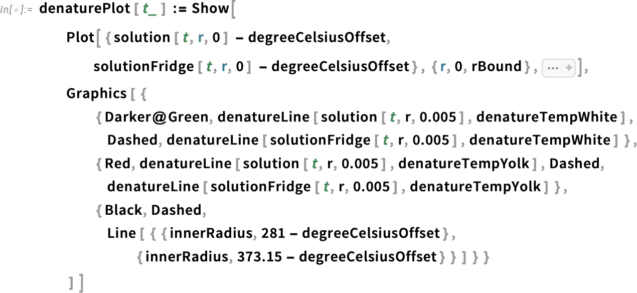
Next, we create a function for the actual plot, where we’re using Show to display the plot and the lines for the denaturation temperatures, calling our denatureLine helper function and also a line indicating the radius of the egg yolk.

Create a helper function to plot the denature positions for the two solutions at various times:

Visualize the temperatures at z = 0.005 for the eggs starting from room and refrigerated initial temperatures and the corresponding denature positions:

Looking at the plot at the six-minute mark, we notice two things. First, it’s clear that the denaturation of the egg white has already reached well into the egg’s center. Second, the denaturation temperature for the yolk has gotten much closer to the center in the case of the room-temperature egg compared with the refrigerated egg.

What does this mean? For the room-temperature egg, the yolk is just starting to cook. But for the refrigerated egg, the yolk is still runny—the denaturation temperature has barely reached the edge of the yolk.

Therefore, if we want a runny yolk, we’ve got two options:

1. Use a refrigerated egg and take it out of the boiling water right at six minutes
2. Use a room-temperature egg and pull it out of the water a few seconds earlier

Visualize the temperatures at z = 0.005 for the eggs at eight minutes:

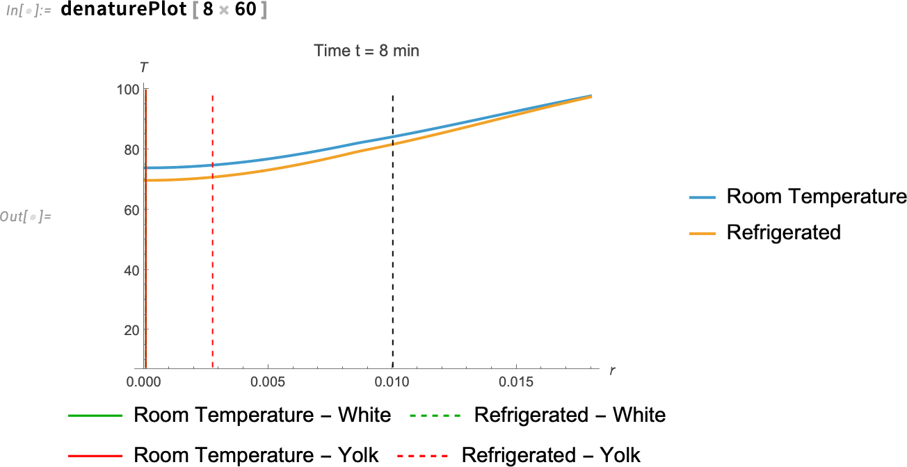
If we make the same plot, but for eight minutes, we see something interesting. At about eight minutes, the entire room-temperature egg has surpassed the denaturation temperature of the yolk, which means that it also has passed the denaturation temperature of the egg white. But there are still some parts of the refrigerated egg’s yolk that haven’t reached that temperature yet.

What does this mean? If you want a fully cooked egg yolk and you’re using an egg straight from the fridge, leave it in the boiling water a few seconds past the eight-minute mark. If you’re using a room-temperature egg—and you’re hungry and don’t feel like waiting—eight minutes may be just enough time.

It All Boils Down to This

We started by creating a simple first version—just something to get our workflow up and running. If we jump straight into coding a complex model, we’re much more likely to make mistakes. What’s worse, those mistakes can be hard to track down. If the results don’t look right, it’s not always clear whether there’s a problem with the model itself or if we just made an error in the code.

By starting simple and gradually adding complexity, step by step, we reduce the chance of introducing bugs. We also get a much better understanding of how our model behaves.

As we saw, the sudden jump in temperature between the outside and inside of the egg was causing numerical issues in one of our early model versions. To fix it, we refined the mesh right at the boundary using a refinement function. This method is much better than refining the entire mesh, since that would slow our computation down significantly.

Finally, we used experimental data in two ways. First, we used experimental data to build our model by setting the parameters in the heat equation. Second, we used the data to compare our results with actual cooking times for real eggs.

We can conclude a few things:

• Creating a simple version first is a good idea.
• Increasing the complexity of the model step by step can make things easier.
• Sharp transitions or discontinuities in solution variables can cause numerical instability or accuracy loss. Use local mesh refinement or smoothing in those regions.
• Having a way to compare our results with real-world data is useful.

Finally, if you found this interesting and want to implement your own PDE models, you can check out this PDEModels Overview in the documentation.