Explore the contents of this article with a free Wolfram System Modeler trial. Have you ever watched Shark Tank or Dragons’ Den? Were you intrigued by the pitches of the founders? After the pitch, you might have heard the sharks or the dragons asking about the growth rate, profit or market size. What do those numbers say about a company? Are losses in the initial years always bad?

I come from an engineering background, so these business questions really intrigue me. To make sense of some of those numbers and how they can give an indication of the future, I decided to model a software-as-a-service (SaaS) company.

For those not familiar with SaaS companies, these are companies that host applications, either locally or on a third-party platform, and provide a service to their customers over the internet. Some popular SaaS companies are Spotify, Netflix and Google Workspace. In fact, SaaS companies have been the fastest-growing sector of the IT industry in the past decade.

For this model, I used the new Version 13.2 of System Modeler, released on December 14, 2022. It has some really cool features like control panels to quickly test scenarios, new Wolfram Language functions to measure system responses and improved resource functions to automatically create dashboards using the control panels. In this blog, you will see that I have made extensive use of these panels.

I will start with an overview of the model, followed by simulations of different strategies, such as the impact of pricing, the result of advertising and the effects of working conditions. Finally, I will introduce you to the concept of the Rule of 40 that angel investors use to judge a SaaS business’s sustainability.

Model of a Sales Funnel

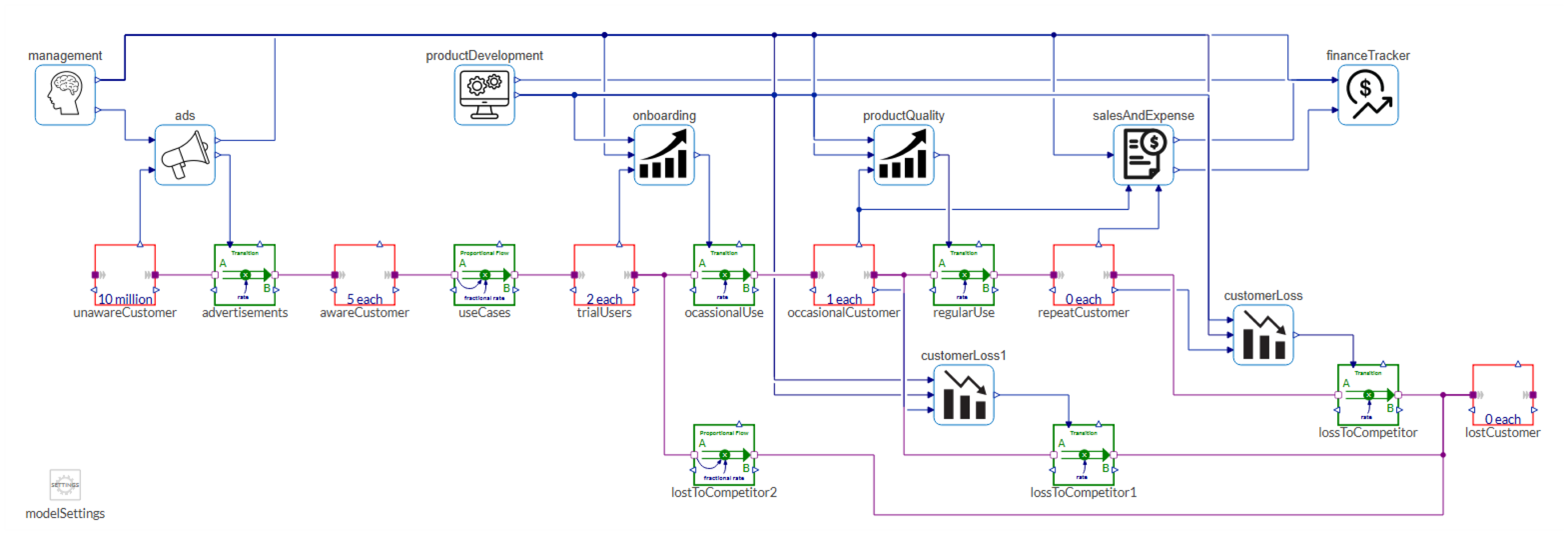
Diagram view of the sales funnel.

I have modeled the process of a customer journey while using a SaaS product. This is called a sales funnel in the marketing lingo. It usually comprises four stages, which are product awareness, interest, decision and action. Sometimes there are also add-ons such as customer loyalty and advocacy.

Let us understand this using an example. Suppose you are browsing through Instagram and you happen to see an interesting post about a smart watch. You don’t realize it, but just by watching that ad you become aware of the smart watch. Then a few days later, say you are watching a documentary on Netflix and you happen to see your favorite celebrity wearing the same watch. You immediately become interested. Then you browse for the watch and find a website where it is sold; you see the cost and compare it with similar watches. You suddenly find that there is a discount code just for the week and you make a decision to buy it. You use the smart watch and happen to enjoy it—you have become a loyal customer. You start talking about the watch with your friends and colleagues, and suddenly you are advocating the watch, thus driving more product awareness.

Stages of a customer journey.

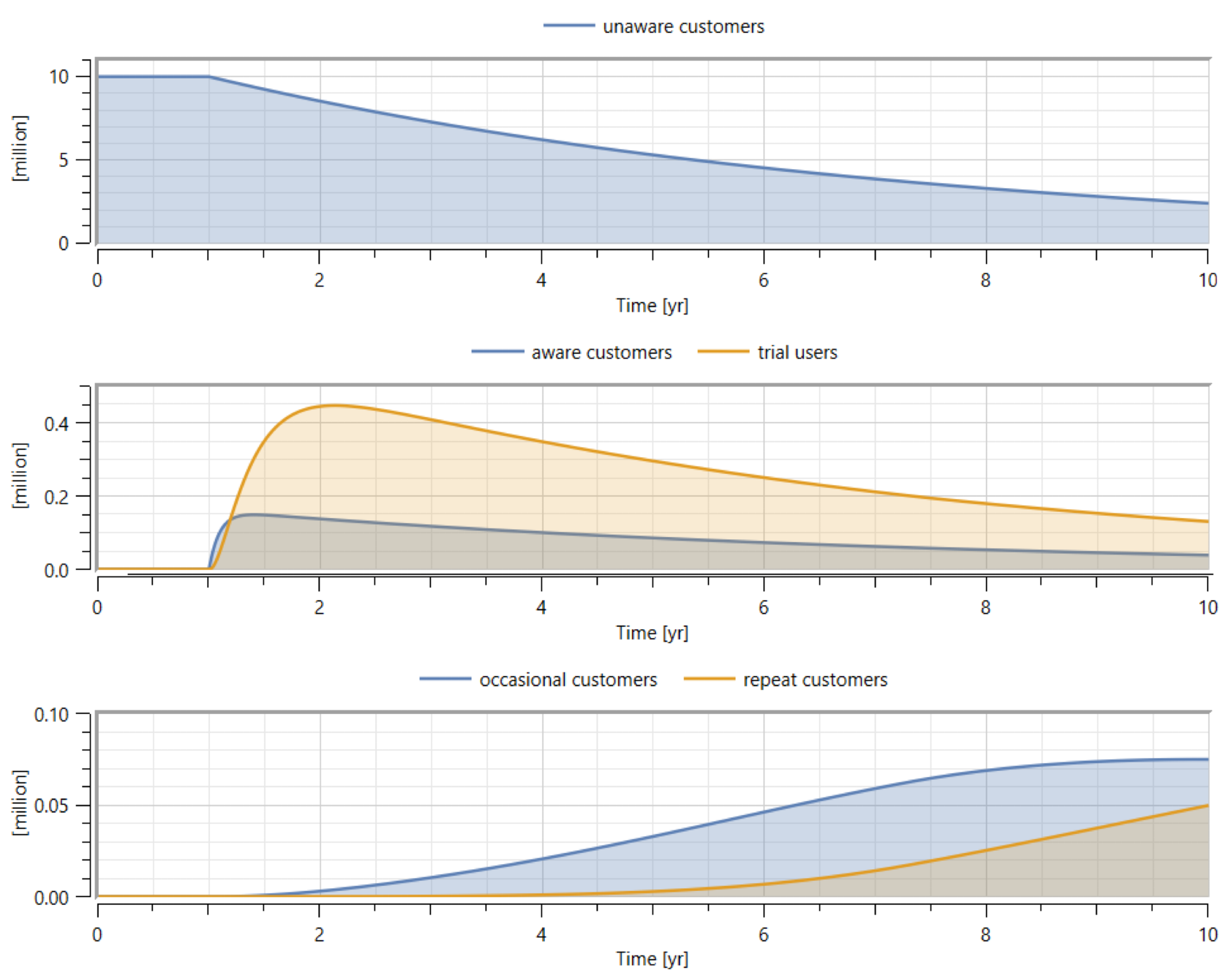
Simulation results of the sales funnel model.

For the preceding SaaS model, the customer journey is similar. They begin in an unaware state, represented by the “unawareCustomer” block on the left. Through ads, people become aware of the product. As they look into more examples, use cases and webinars, they become interested and become trial users. If they find the product trial to be useful, customers may then select a one-time subscription and cancel after the first billing period. And finally, as they start using the product more, they hopefully find it helpful enough to keep using it regularly and become repeat customers. Of course, during their journey, there can be negative experiences or better product offerings from competitors, and people may quit the brand.

In case you are wondering what those purple and green blocks are, they are called stocks and flows. Stocks are like water containers, while flows are like pumps that control the rates of their in- and outflows. This idea was envisaged by Jay W. Forrester and its domain is known as system dynamics. For this model, I have made use of the free Business Simulation library, which contains pre-made blocks that you can use simply by dragging and dropping. More information about the library and system dynamics can be found in this blog.

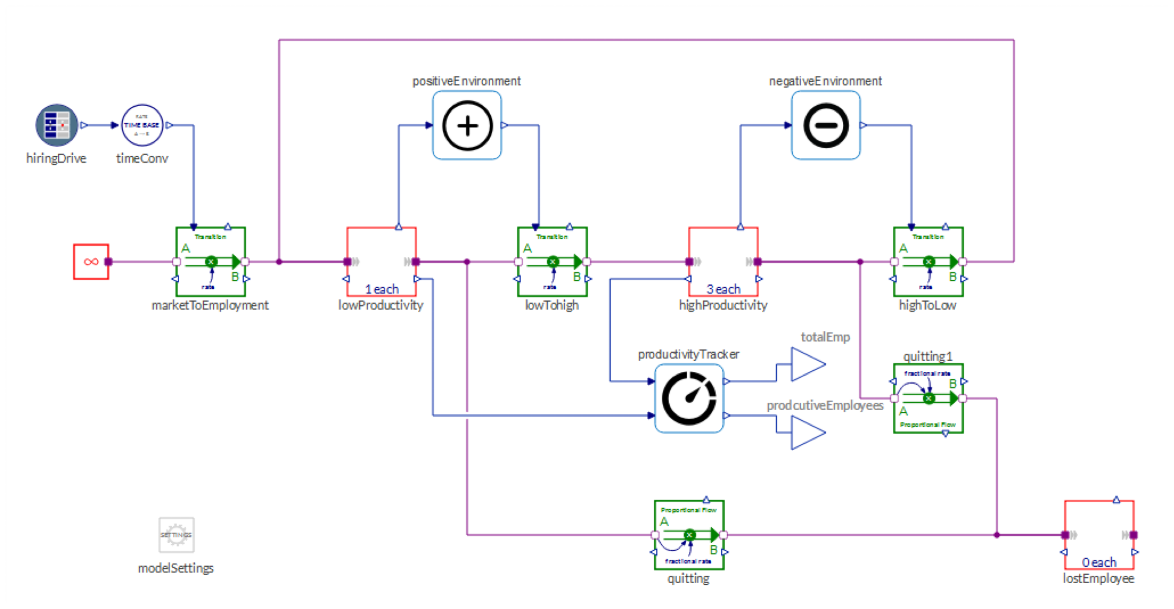
Diagram view of the employee productivity component.

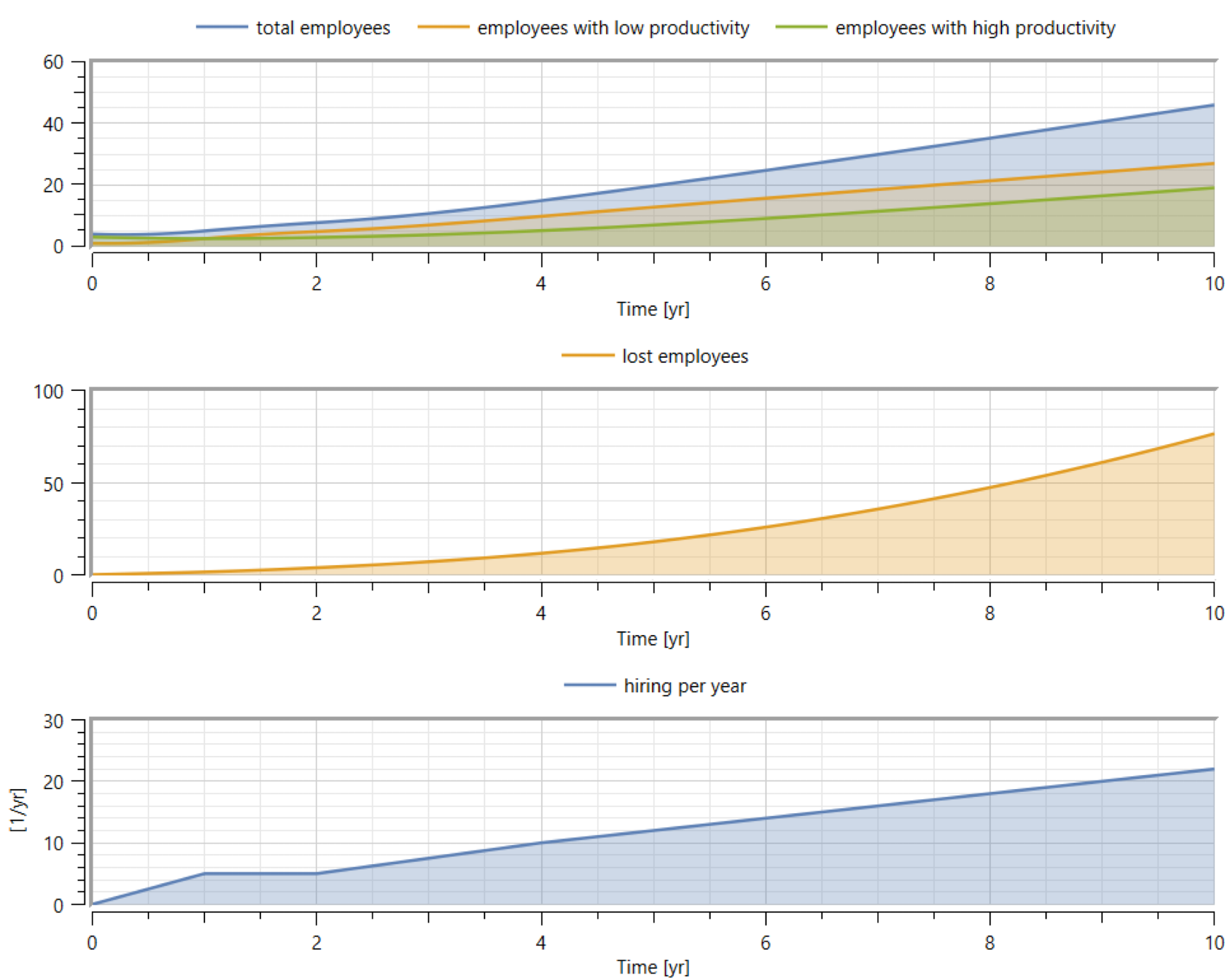
Simulation results of the employee productivity component.

The sales funnel model also consists of components like product development, employee productivity and more. The previous figure shows one of the submodels for estimating the productivity levels of employees. Once hired, employees need time to adapt to the new work environment and do not produce at their peak levels. With proper training and support, they become experts and thus more productive. However, there is also the possibility that due to stress and burnout, a productive employee loses motivation and reverts to an unproductive stage.

For the sake of brevity, I will not explain the other components. You can download a trial version of System Modeler and check them out. The blocks used to create them are the basic stock and flow blocks and some math blocks like gain, add, clip, etc.

Of course, my model does not cover all the details of a SaaS company, like rent and other miscellaneous expenses, nor does it consider the loss of customers due to a competitive market. The purpose of my model is to get a general trend by incorporating some first principles. Let’s begin to test some strategies.

Modeling a Pricing Strategy

In the model, the transition rates of customers, from trial users to occasional customers to repeat customers, are inversely related to the product price, whereas the loss rates of customers to competitors are directly related to the product price.

Let’s check a traditional pricing strategy. Here, the product price is constant. The company incurs some losses at the start as it spends heavily on advertising and product development. At the end of the simulation, the company makes an accumulated profit of seven million sharks (I am using sharks as the unit of money in this qualitative model) with a total customer base of one hundred thousand.

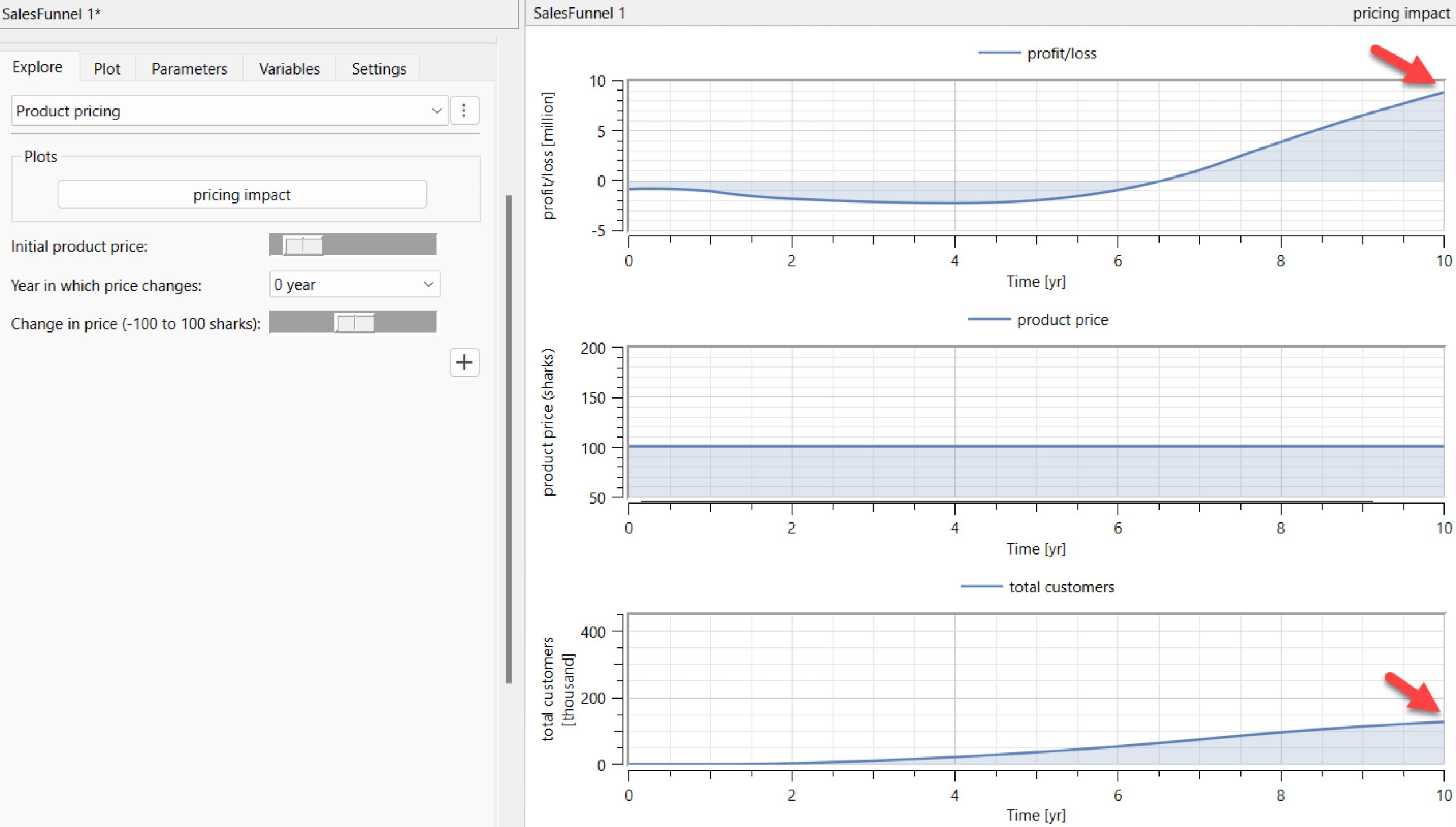
Simulation results of a traditional pricing strategy.

If you have used previous versions of System Modeler, you might notice that now you can add sliders, popup menus and other control objects in the Explore tab on the left in Simulation Center. This makes it really convenient to test different scenarios as well as provides a nice interface for model users. You can attach a plot (like the “pricing impact” plot) for quick reference or add multiple interfaces (called panels) to a model. In the sales funnel model, I have added three panels, “Product pricing,” “Employees,” and “Advertising.” Watch this video to see how easy it is to create such interactive panels.

Now, let’s try a new strategy. We will start selling the product at a very low price. As the product is very cheap, a lot of people buy it. After five years, we drastically increase the price of the product. This reduces the transition rate of customers from trial users to paid customers, and also increases the loss rate of customers to competitors. However, as some customers have started to use the product regularly, they will find it difficult to stop using it completely. For example, let’s say you have a few GBs of data in a mail service like Gmail, and suddenly they decide to start charging for their service. As you have so much dependency on it already, you decide to pay the charges and keep using it. At the end of the simulation, the accumulated profit is around 70 million sharks with a total customer base of four hundred thousand.

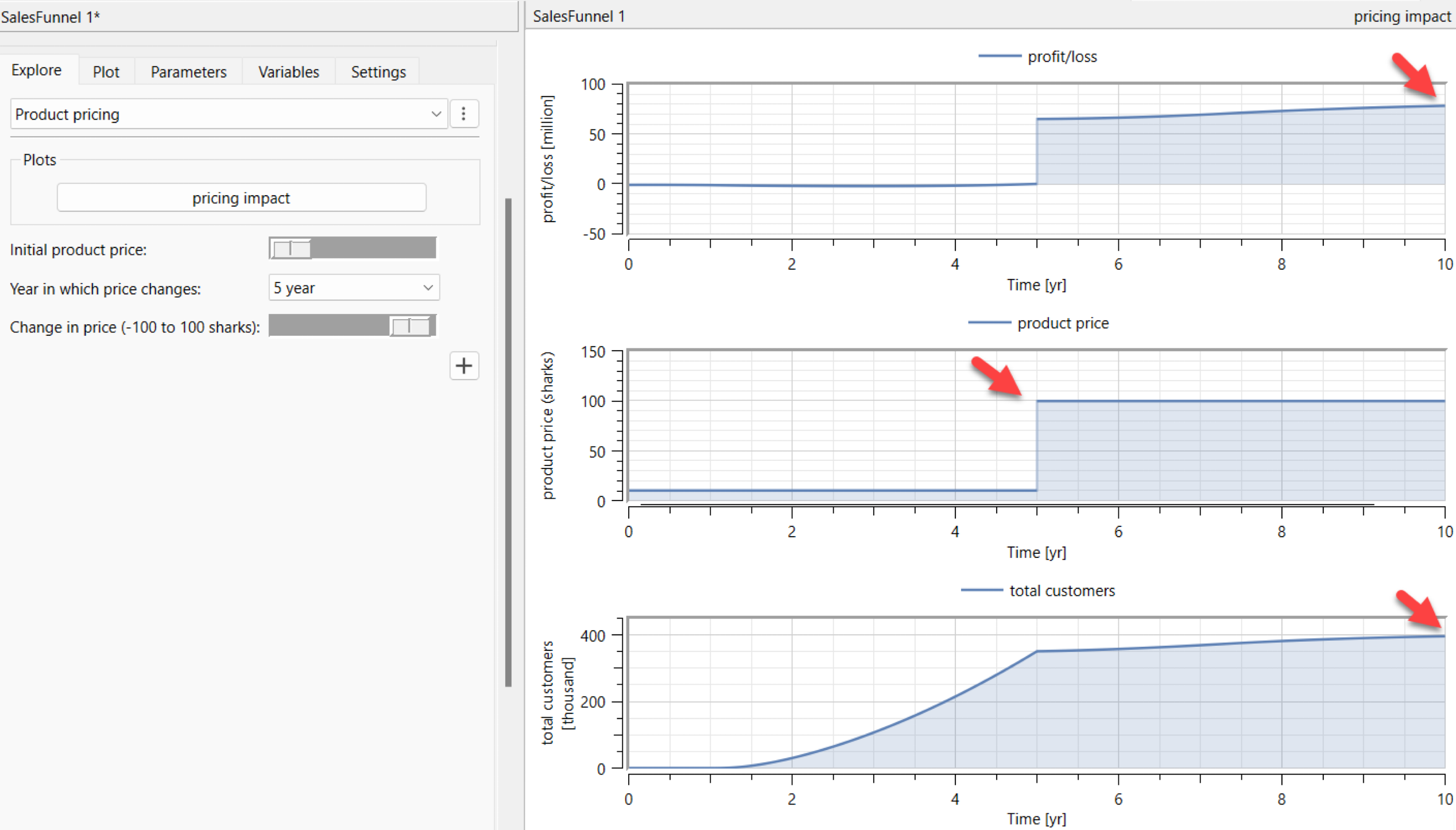
Simulation results of the new pricing strategy.

Visualizing an Employee Onboarding and Attrition Management Plan

How will the onboarding process and attrition management policy affect performance? When employees join a company, it is very unlikely that they will have the required skills and knowledge of standard operating procedures (SOPs) to be productive from day one. It will take time until they reach their peak productive levels. That duration would depend on the effort put into training and good working conditions like supportive colleagues. Similarly, with a poor attrition management policy, a company keeps losing productive employees and ends up with a major share of new employees who are not that productive.

For the exploration of this strategy, we will switch to the “Employees” panel. To keep the parameter values qualitative, I have used labels like “low,” “average” and “high” rather than absolute values for the training quality and attrition parameters. These labels are attached to different transition rates. The training quality controls the transition from the low-productivity stage to the high-productivity stage, whereas the attrition parameters control the quitting rates.

Let’s set the training quality to “average” and attrition to “high.” By an “average” training quality, I mean that the company has not defined a training path for its new employees, and as a result they acquire the necessary skills in bits and pieces. With “high attrition,” I mean that there is no attrition management policy in place. No special effort is taken by the company either by financial incentive or improving the working conditions to control the attrition rate. The simulation shows that at the end, there are about 35 employees left in the company, with most of them being in the low-productivity stage and only a few in the high-productivity stage. The company has produced about 200 thousand product man-hours at an expense of 7 million sharks—that is about 35 sharks per productive man-hour.

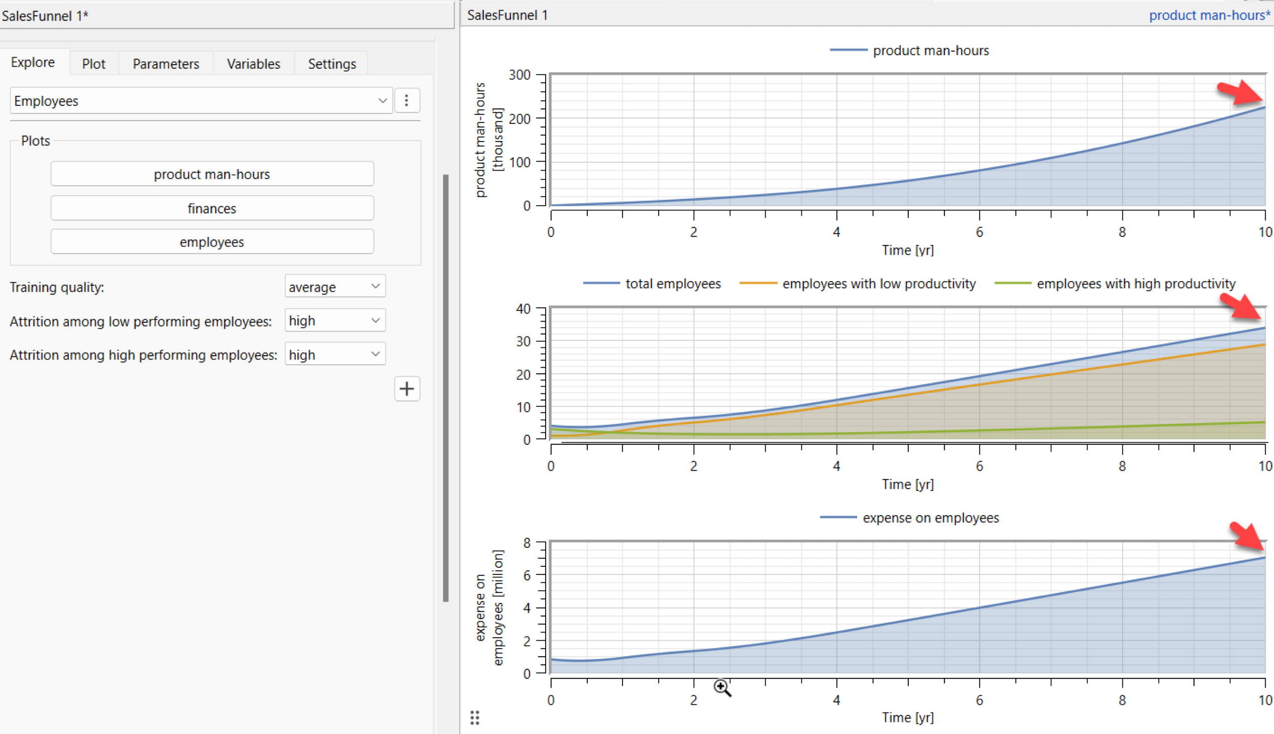
Simulation results with training quality set to “average” and attrition set to “high.”

Now, let’s put a carefully designed training program in place (training quality set to “best”) and take an additional effort in retaining employees (low attrition). The simulation shows that there are about 70 employees left in the company, with a majority of them being in a high-productivity stage. The company has produced about 450 thousand product man-hours at an expense of 15 million sharks; that is about 33 sharks per productive man-hour. So a good employee onboarding and attrition management plan has resulted in a better product (I am assuming more man-hours spent on the product will lead to a less buggy and more feature-rich product) along with cost savings.

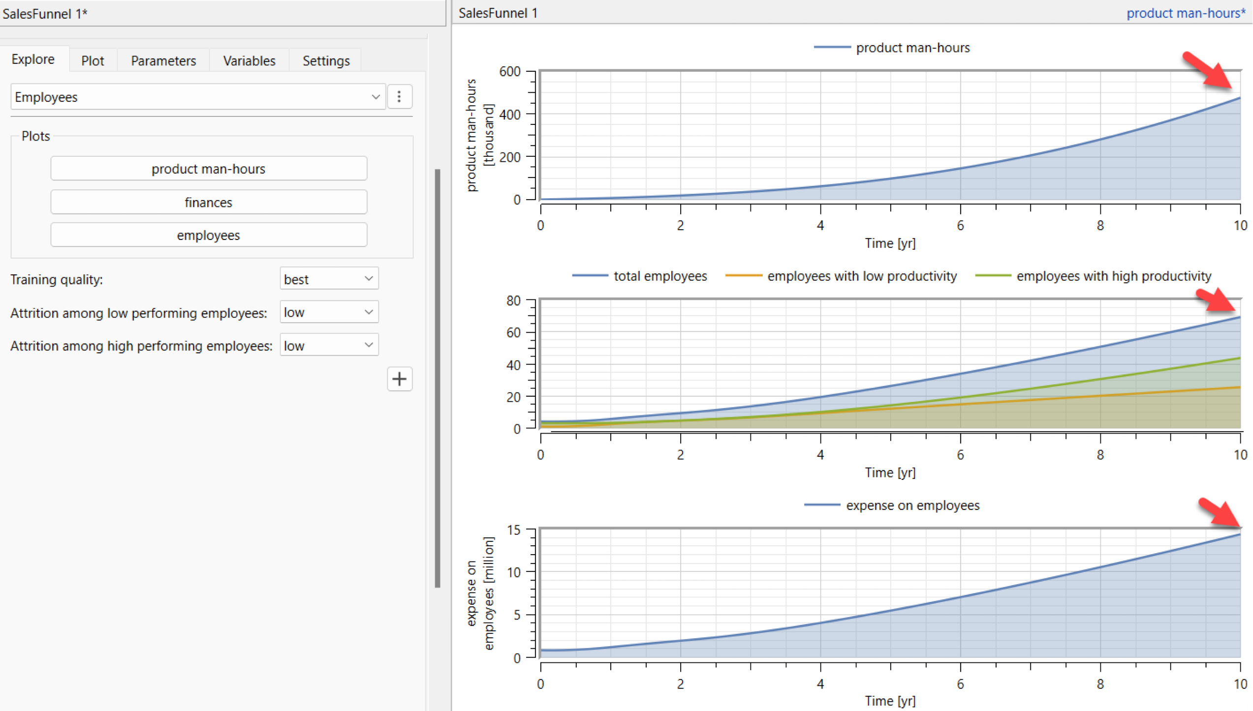
Simulation results with training quality set to “best” and attrition set to “low.”

Maximizing Paid Advertising

Should a company constantly spend money on ads, or can it stop investing after advertising for a certain period of time? In the model, the advertising funds are solely used for social media ads that convert unaware customers to aware customers.

We will switch to the “Advertising” panel for this strategy and use the “advertisements” plot. I use a square wave to define the advertisement fund distribution. You can set the start and stop years as well as the offset (used to define the advertisement budget). There is also a parameter to set the advertisement channel impact; this defines how effective the social media platform is. For instance, a high-impact label means a higher transition rate from unaware customers to aware customers.

In this strategy, we will spend five hundred thousand sharks every year from year 1. In the end, the company reaches an accumulated profit of eight million sharks. However, there is also an interesting behavior to observe in the middle plot, which tracks the number of ad impressions, i.e. ad views. You can see that the number of ad impressions is going down. This is because it becomes gradually harder to reach new unaware customers (new market) with a constant amount of yearly spending.

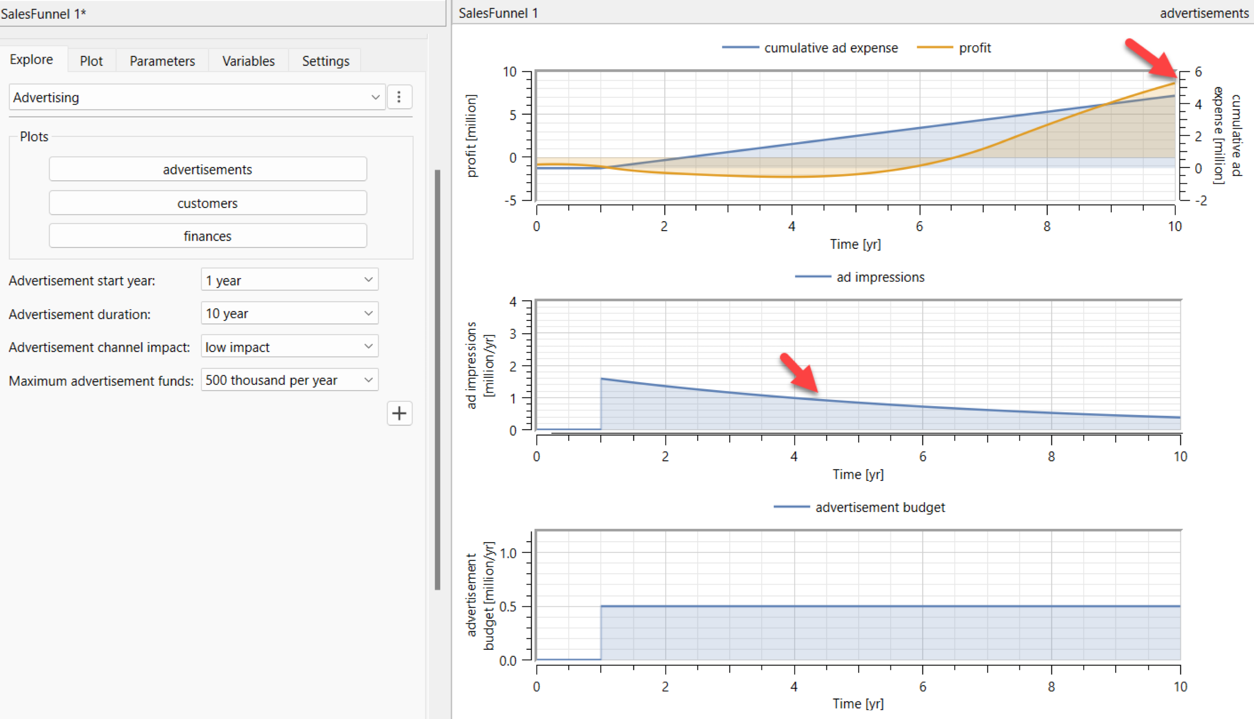
Simulation results with fixed advertising budget from year 1.

Now we will spend more and stop after five years. You can see that as we stop the spending, our accumulated profits start to grow, but they eventually plateau and we make no accumulated profit at the end. Perhaps it is a good strategy to invest regularly rather than irregularly.

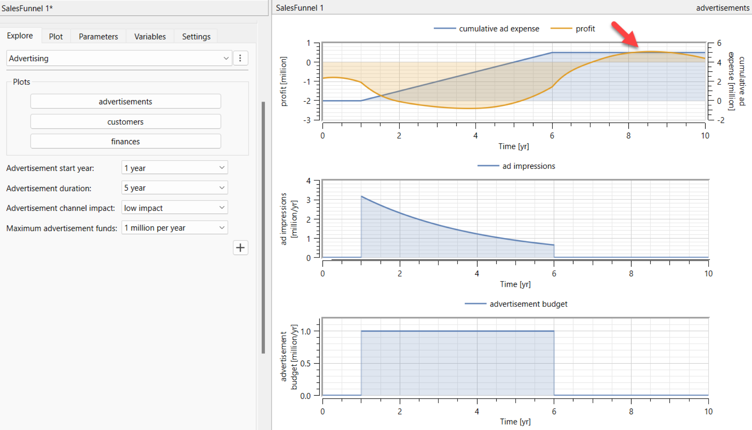
Simulation results with a fixed advertising budget from year 1 to year 6.

Funding: The Rule of 40!

There is a concept in the investment community for SaaS companies called the Rule of 40. It means the average revenue growth rate plus profit margins should be more than 40% for the business to be considered sustainable.

We will use the new SystemModelMeasurements function to find the growth rate between years 4 and 5. The function is especially useful when you work with designing controllers. It can help you quickly find your system’s control performance. Using it the way I have here is trivial, but I find it easy to obtain values this way.

You will need a compiler to run system modeling functions. Check this resource article for more information.

Engage with the code in this post by downloading the Wolfram Notebook

&#10005

&#10005

&#10005

&#10005

&#10005

Our model has an annual revenue growth rate of about 62% between years 4 and 5, and the profit margin is –34% in year 5. So according to the Rule of 40, the sum of the annual growth rate and profit margin is 28%; thus, it does not reach the minimum requirement of 40%.

Share the Results

Now that we have tested some strategies, we would like to share the results so that others can play around with them. One way to do this is by sharing this notebook using the Wolfram Cloud. Even though the Wolfram Cloud does not have the graphical interface of System Modeler, we can still use it to distribute the model results as a dashboard.

We will use the SystemModelManipulate resource function to automatically generate the dashboard using the control panels that I stored in the model.

&#10005

I hope this blog gave you an idea of how modeling can help in simulating trends and enables you to understand how the various subcomponents interact with each other. If you have ideas on how I can improve my model, please feel free to comment below.

Learn More

You can download the model here. You will need to install the free Business Simulation library to run it. If you want to learn more about the new features of System Modeler 13.2 and the Business Simulation library, do check out the following links:

• What’s New
• Business Simulation library

Need help implementing a computation-based project? Talk to our Technical Consulting team about your project.