What is the half-derivative of x?

Fractional calculus studies the extension of derivatives and integrals to such fractional orders, along with methods of solving differential equations involving these fractional-order derivatives and integrals. This branch is becoming more and more popular in fluid dynamics, control theory, signal processing and other areas. Realizing the importance and potential of this topic, we have added support for fractional derivatives and integrals in the recent release of Version 13.1 of the Wolfram Language.

The Idea of Fractional Calculus

The foundations of calculus were developed by Newton and Leibniz back in the seventeenth century, with differentiation and integration being the two fundamental operations of this subject.

Every student of calculus knows that the first derivative of the square function is x, while the result of integrating it is and that integration is essentially the inverse operation of differentiation (the integral of order n may be regarded as a derivative of order –n). However, speaking about derivatives or antiderivatives or integrals, we assume the order n is integer.

Engage with the code in this post by downloading the Wolfram Notebook

&#10005

What if the ideas of differentiation and integration could be extended to noninteger or even complex orders? This is done in the theory of fractional calculus, which generalizes the classical calculus notions of derivatives and integrals to fractional orders α such that the results of fractional operations coincide with the results of classical calculus operations when the order α is a positive integer (differentiation) or negative integer (integration). As shown in the following illustration, derivatives of other real orders “interpolate” between the derivatives of integer orders:

&#10005

Historical Overview

Fractional calculus is not a new subject. It has at least a two-century history starting from the two articles written by Niels Henrik Abel back in 1823 and 1826.

As explained in this article, fractional calculus was introduced in one of Abel’s early papers, where all the elements can be found: the idea of fractional-order integration and differentiation; the mutually inverse relationship between them; the understanding that fractional-order differentiation and integration can be considered as the same generalized operation; and even the unified notation for differentiation and integration of arbitrary real order.

&#10005

Abel considered the generalized version of the tautochrone problem (also known as Abel’s problem) on how to determine the equation for the curve KCA along the slope from the prescribed transit time T = f(x) given as a function from the distance x = AB.

Abel obtained the integral equation for the unknown function φ(x), the determination of which makes it possible to find the equation for the curve itself. After several algebraic manipulations, this integral equation might be rewritten in the form 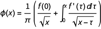, which is what we call now the Caputo fractional derivative.

During the last two centuries, scientists from different areas and backgrounds worked on the theory of fractional calculus (considering it from different points of view). Hence, there are different approaches on how to define a fractional “differintegration” operation. Three of these definitions are the most popular and important in practice. We will talk about them in this blog post.

Half-Derivative of the Square Function

Let’s take the square function and derive the formula for the fractional derivatives using some simple algebraic manipulations. First, let’s calculate the n^th-order ordinary derivative of the square function:

&#10005

Putting negative n in this formula, one might easily get the n^th-order antiderivative of this function:

&#10005

Let’s take the formula for the n^th-order derivative of the square function and put a noninteger order n into it:

&#10005

And what will we get if we take the n^th-order ordinary derivative of the latter function and substitute 1/2 there?

&#10005

This is the first derivative of the square function! It is obtained via two “half-order fractional differentiation” procedures. One might easily verify that the antiderivative of the square function can be obtained via two similar half-order integration procedures (substituting –1/2 in the previously shown formulas).

So with this simple example, we show what fractional calculus is and how it is connected with as well as how it generalizes the classical version.

Three Main Definitions of Fractional Derivatives

As integration is essentially the inverse operation of differentiation, we could define one united operation of differentiation/integration, which we call the differintegral: in the literature, this operator is written as , which stands for a fractional differintegral of order α of the function f(x) with respect to x and with the lower bound a. Fractional differintegrals depend on the value of the function f(x) at the point a so they use the “history” of the function. In practice, the lower bound is usually taken to be 0.

Grünwald–Letnikov Approach

The Grünwald–Letnikov differintegral gives the basic extension of the classical derivatives/integrals and is based on limits:

In practice, this approach is not very usable, as it contains an infinite number of approximations of a function at different points.

Riemann–Liouville Approach

The Riemann–Liouville definition is:

, where

It lies under a solid and strict mathematical theory of fractional calculus. This theory is well developed, but the Riemann–Liouville approach has a couple of limitations that make it not so suitable for applications in real-world problems.

Caputo Approach

The Caputo definition is:

, where

There is some similarity between this and the Riemann–Liouville differintegral and, in fact, the Caputo differintegral can be defined via the Riemann–Liouville differintegral:

Obviously, for negative α, the Caputo fractional derivatives coincide with the Riemann–Liouville fractional derivatives.

The Caputo definition of fractional derivatives and integrals has many advantages in comparison with the Riemann–Liouville or Grünwald–Letnikov ones: first, it takes into consideration the values of the function and its derivatives at the origin (or, in general, at any lower-limit point a), which automatically makes it suitable for solving fractional-order initial-value problems using Laplace transforms. Also, the Caputo fractional derivative of a constant is 0 (while, in general, the Riemann–Liouville fractional derivative is not), hence it is more consistent with classical calculus.

The following animation shows the behavior of the Caputo fractional derivatives of a square function in comparison with the ordinary ones—the fractional-order derivatives “interpolate” between the derivatives of integer orders:

&#10005

Riemann–Liouville Fractional Differintegral in the Wolfram Language

We have implemented a function called FractionalD into Wolfram Language Version 13.1. This function computes the Riemann–Liouville fractional derivative of order α of the function f(x).

As an example, let’s calculate the half-order fractional derivative of a cubic function:

&#10005

Now verify this result using the Riemann–Liouville definition:

&#10005

Repeating the half-order fractional differentiation procedure leads to the ordinary derivative of the cubic function:

&#10005

The following calculation recovers the initial function using three nested fractional integrations:

&#10005

Now let’s compute the arbitrary fractional-order derivative of this cubic function, make a table of its values for specific orders and plot the list of derivatives:

&#10005

&#10005

&#10005

Next, let’s compute the 0.23-order fractional derivatives of the Exp and BesselJ functions:

&#10005

&#10005

Here, we show the fractional derivative of the MeijerG superfunction, as it is a very important theoretical case: the fractional derivatives of MeijerG are given in terms of another MeijerG function:

&#10005

As a final example, we present a table of the α^th fractional and n^th ordinary derivatives for a few common special functions:

&#10005

Caputo Fractional Differintegral

In Wolfram Language 13.1, CaputoD gives the Caputo fractional derivative of order α of the function f(x).

As mentioned previously, the Caputo fractional derivative of a constant is 0:

&#10005

&#10005

For negative orders of α, the CaputoD output coincides with FractionalD:

&#10005

&#10005

Now, let’s compute the 0.23-order Caputo fractional derivative of the Exp function:

&#10005

Compute the half-order Caputo fractional derivative of the BesselJ function:

&#10005

And as a final example, we present the half-order Caputo fractional derivatives of some common mathematical functions:

&#10005

Fractional Differential Equations

Fractional differential equations (FDEs) are differential equations involving fractional derivatives d^α l d x^α. These are generalizations of the ordinary differential equations (ODEs) that have attracted much attention and have been widely used in engineering, physics, chemistry, biology and other fields. In most of their applications, FDEs involve relaxation and oscillation models.

Here is an example in which we solve an FDE using the powerful DSolve function, which was heavily updated in Version 13.1 to support FDEs:

&#10005

This solution is given in terms of the MittagLefflerE function, which is the basic function for fractional calculus applications. Its role in the solutions of FDEs is similar to the role and importance of the Exp function for the solutions of ODEs: any FDE with constant coefficients can be solved in terms of Mittag–Leffler functions.

Now, let’s plot the previous solution:

&#10005

As a more interesting example, we solve the equation of a fractional harmonic oscillator of order 1.9:

&#10005

The behavior of this fractional harmonic oscillator is very similar to the behavior of the ordinary damped harmonic oscillator:

&#10005

Plot these solutions and compare them:

&#10005

This example clearly demonstrates that the order of FDE can be used as a controlling parameter to model some complicated systems.

Another method for solving FDEs is via the Laplace transformation of the equation (i.e. transforming the initial FDE to some algebraic equation). We’ve also added LaplaceTransform support for FDEs in Version 13.1:

&#10005

Now, calculating the inverse Laplace transform of this solution, we will immediately get the same solution obtained via DSolve:

&#10005

Closing Words and Acknowledgments

Here at Wolfram Research, we are constantly updating the Wolfram Language, covering more and more topics that could be revolutionary and push scientists to start innovative research in their areas of study.

In Wolfram Language 13.1, we have implemented two basic operators for fractional calculus (the FractionalD and CaputoD functions), and also made a huge effort to add support for solving fractional differential equations via DSolve and LaplaceTransform. We have also updated the algorithms of the MittagLefflerE functions, as they have crucial importance in the theory of fractional calculus. You can learn more about this from both the blog post “Launching Version 13.1 of Wolfram Language & Mathematica” by Stephen Wolfram and the New in Wolfram Language 13.1 webinar series.

Also, I would like to acknowledge the work done by my colleagues Aram Manaselyan and Hrachya Khachatryan on the implementation of fractional calculus in the Wolfram Language; the invaluable contribution of Professor Oleg Marichev to the theory of fractional calculus and symbolic computational algorithms within it; and Devendra Kapadia for managing the project as well as for valuable remarks and critical comments on this text.