What Does Hollywood Have to Do with the Chicken Head?

In a relatively popular marketing device in the past decade, chickens found their way into online advertising and TV commercials, where their impressive focusing and stabilization skills were displayed. Hold them gently and then move them up, down or rotate them slightly, and their eyesight stays at a constant level.
How do we build a device that mirrors those features? To find out, let’s embark on a journey from car suspensions to camera stabilization systems that reaches for those standards of excellence in engineering that can only be described as “majestic as the chicken.”
A Chicken Is Like a Spring
The first challenge we face is modeling such a system. An engineer could write a set of equations and plug them into a solver, but even for a relatively small model, this can produce a lot of results that are hard to share and visualize with peers because you can easily end with unconventional variable names, parameter choices and unit conventions.
Explore the contents of this article with a free Wolfram System Modeler trial.Given the choice, we would rather go to Wolfram System Modeler and use physical component–based modeling. If we want this model to have, say, a spring, then we drag a spring component and drop it on our canvas. We don’t have to remember equations from college, and we get the added benefit of built-in animations.
It is not by accident that we mentioned springs. When we see a chicken’s neck expand and contract to stabilize its eyesight, it’s the first thing that comes to mind. A physicist would say that in a spring, energy that comes from motion is stored in the spring itself, but some could also be lost, depending on the amount of elasticity and dampening the system has.

This observation is what allows us to model structures that we parameterize in terms of how they handle incoming input energy, with part of that energy being stored and a part being lost. With this approach, we can build more complicated objects by putting together subsystems with different types of responses to inputs. Adding just the right elastic and dampening parameters can take us far on the path to modeling and controlling real systems.
Assembling the Model
Let’s make a simple model for the disturbances and dynamics involved in the stabilization of vertical motion. The system we use to mimic the response of the chicken is a camera mounted on top of a car. The disturbances caused by the road will transmit energy to the car and the camera. The objective for us is to design a control system that will negate those disturbances and allow us to have a smooth response.
We start by assembling a model of the system. We can emulate the interaction between the road, the car and the camera by connecting several spring-mass systems in series, each on top of the other. With the camera at the top, we let this system be affected by gravity, and we add two inputs. One represents the disturbance force, which acts from the bottom. The other one is a control input acting on the camera that will allow us to represent the device that stabilizes our recording setup.
(Download the model we created so you can evaluate the code in this post. Just make sure you save it to the same directory as the Wolfram Notebook you’re using.)
Analyzing the Model
How do we know if we have made good choices for our parameter values? Let’s run some simulations and check that the results make sense. We start by importing the model:
 Engage with the code in this post by downloading the Wolfram Notebook

✕
|
If we ask for input variables, we get the disturbance force fw and a control input fa as inputs:

✕
|
To improve camera performance, we need either a person or a device to hold the camera steady. We can skip the former because no human being is a match for a chicken’s reflexes. That’s the reason we have the actuator fa that is placed between the camera and the car body.
While controlling the camera position, we need some measurements that will help us determine how much force we need to apply to get the camera to its desired place. Two potentiometers can be a good fit for this job: one between the car tire and the body and the other one between the car body and the camera. These are the two outputs, ycb and ywb, of the model:

✕
|
The state variables are the deviations of the car (xbe), wheels (xwe) and camera (xce) with respect to their equilibrium positions and their velocities:

✕
|
We can see all these variables again when computing a linear state-space representation of the model:

✕
|
If we give the system a sudden bump of 2000 N, our uncontrolled system oscillates very badly:

✕
|
The camera jumped more than two centimeters!
Designing the Controller
By mimicking the mighty chicken, we got a system composed of a car and a camera. Its performance is way worse, however, than the chicken’s. It is time to control the camera position so that we can get better shots.
What control design can we implement? We can start by studying the poles of the system. For a linear system, these can be found by taking the state matrix and computing its eigenvalues, which will be complex numbers. The poles of the system play a crucial role because they have a big say in the characteristics of the system’s response.
It can be roughly claimed that the poles should always be on the left side of the complex plane. This condition guarantees that the structure will be stable. The further to the left the poles are, the better stability we have. We do not know precisely, however, which poles should be chosen. In other words, where should we draw a line, and which criteria should we apply?
Let’s consider the control effort. According to the chosen poles, the camera stabilizer force varies. If we want to have a quicker response, we need to aim for poles further left in the s plane. But this costs us more control effort. Thus, we have a tradeoff between the performance and the control effort.
The linear quadratic (LQ) controller technique helps us to express this tradeoff mathematically as an optimization problem that minimizes a cost function of the form  . Here, x(t) and u(t) are state and input variables, and q and r are weighting matrices that capture the tradeoff. A small q matrix or large r matrix penalizes the states and will result in a controller that will produce a quick response at the expense of a larger control effort. On the other hand, a large q or r matrix penalizes the inputs and will result in a controller with a slower response and a smaller control effort.
The solution of the optimization problem is a simple linear equation of the form u*(t) = –k.x(t). Here, u*(t) is the optimal value of u(t) and k is a matrix of appropriate dimensions.
We have a built-in function, LQRegulatorGains, that has been recently updated to directly handle SystemModel objects and to automatically assemble the closed-loop system.
But how do we go about assigning values for the q and r matrices for this system? We can try and attenuate the whole system, including the vibrations in the tires and the car body. This would result, however, in an exorbitant control effort. Instead, let’s focus on attenuating the vibrations of just the camera.
The camera’s position (xce) and velocity states (vce) are the second and third states:

✕
|
We will assign large values for the weights corresponding to these two states and have the values for the other states and the control input at a much lower value:
;r = ({ {1} });")
✕
|
Now, compute a controller using these weights:

✕
|
We asked for the data object, so LQRegulatorGains returns a SystemsModelControllerData object. This object can be used to query or compute several properties of the designed controller and closed-loop system:

✕
|
Let’s look at the computed controller, which is typically of the form –k.x:

✕
|
In accordance with the specified weights, we see that the second and third states, which are the camera’s position and velocity, have the most influence on the control effort, while the third and sixth, which are the wheel’s states, have the least effect.
The closed-loop model of the original model with the controller can be easily computed using ConnectSystemModelController:

✕
|
We can then simulate it:

✕
|
Take a look at its responses:

✕
|
From the previous plot, it’s difficult to make out the camera’s response, which appears flat. So we’ll plot just that:

✕
|
The camera on the uncontrolled system originally had 2 cm oscillations, and now that has been reduced by a factor of 104!
Let’s check the control effort as well:

✕
|
It is less than 4 N, and it is a practical and cost-efficient control.
The weights q and r that were used previously were arrived at after a series of iterations. As we tweaked the weights, we evaluated the system’s performance and the control effort. The notebook is quite a handy interface to carry out these explorations and record the values that look promising for further refinement and analysis.
Analyzing the Controller
Let’s analyze what the controller did to the system.
The uncontrolled system has a very oscillatory mode:

✕
|
Now let’s look at the modes of the controlled system:

✕
|

✕
|
Notice that we have excluded the leftmost pole in the last plot to zoom in on the more interesting remaining ones. Two of the modes are essentially untouched, especially the seemingly problematic one that is closest to the imaginary axis. What the LQ controller did was to attenuate that mode’s response but did not remove the oscillations. That’s why we see those small oscillations up to 10 seconds, similar to the uncontrolled system.
What happens if we try to dampen that dominant mode a bit faster?
To do this, we are going to use the pole-placement approach to compute the previous gain matrix k. This is a single-input system, so the solution to the controller problem is unique and both the pole-placement and optimal LQ techniques will give the same result.
These are the poles of the closed-loop system that will not be changing:

✕
|
We’ll create a function that will take the new eigenvalue, join it with the rest, compute the new controller and plot the new system responses and controller effort:

✕
|
If we leave the dominant mode unchanged, we should get the same response as the LQ design:

✕
|
If we try to move this mode ~0.02 rad/s, the control effort increases by a large factor:

✕
|
If we move 0.2 rad/s, the control effort increases even more:

✕
|
What we observe is that the oscillations in the controlled camera, although attenuated significantly, cannot be damped out without significantly increasing the control effort. The LQ design achieved a good balance, however, between attenuating the oscillations and keeping the control effort feasible.
Designing the Estimator
The controller we designed depends on the values of the positions of the three masses and their velocities. Using six measurements directly would not only require the same number of sensor readings but would also not compensate for any errors or noise in the readings. So we’re going to use an estimator to provide the required values to the controller.
An estimator uses a set of measurements and the model of the system to estimate the values of the states. For example, we can estimate the number of people in an office building at any given time by counting the number of cars in its parking lot.
In our case, the two measurements are the relative positions of the camera and tire with respect to the car body:

✕
|
ObservableModelQ tells us that it’s possible to estimate the states from these two measurements and the model:

✕
|
We are going to use the pole-placement approach to design the estimator. This works just as in the case of the controller, except that we’re placing the estimator’s poles. If we place the estimator’s poles well to the left of that of the controller’s, the errors between the actual and estimated values will decay fast. The following are the closed-loop poles:

✕
|
After a few trials, we ended up placing the poles of the estimator at the following locations:
|
✕
|
We then use the function EstimatorGains, which implements the pole-placement algorithm and computes the observer’s gains:

✕
|
The estimator itself is a dynamical system, and the system is connected to the controller and estimator as shown here:

✕
|
We don’t have to do any assembling manually. Instead, we can use the function EstimatorRegulator to do that—and much more!—for us:

✕
|
We can query the data object for the estimator model if needed:

✕
|
But what we are really after is the complete closed-loop system:

✕
|
Let’s now simulate the closed-loop system to see how well the system with the estimator and controller performs:

✕
|
If we take a look at the system states, it appears to have responses similar to what we got without the estimator:

✕
|
The control effort is also comparable to the controller without the estimator:

✕
|
The response of the camera is now well damped, but it has a transient jump that quickly dies out:

✕
|
Comparing it with the uncontrolled camera, we see that all the oscillations have been eliminated and the camera stabilized after a quick initial transient:

✕
|
Improving Performance
Improving the performance of machine learning models often requires exploring the space of hyperparameters, metrics and data processing options. In a similar fashion, improving the performance of controllers requires testing and analysis. The key aspect when doing either is to have a framework where this investigation becomes natural and easy.

With an approach based on physical modeling in System Modeler, an expanding and continuously improving control systems functionality in the Wolfram Language, and their seamless integration, we have a framework of streamlined and powerful tools for modeling and controller design. And this is not the end of the line for them!
In this blog, we have shown these tools in action. We encourage you to try these out for the systems you want to investigate and design. For more information, explore the many domains covered in the Modelica Standard Library, our tech note on getting started with model simulation and analysis, our guide on system model analytics and design and our guide on control systems.
| Check out Wolfram’s System Modeler Modelica Library Store or sign up for a System Modeler free trial. |

Comments