Generative Adversarial Networks (GANs) in the Wolfram Language
 in the Wolfram Language")
A noteworthy achievement of artificial intelligence, since it is driven by artificial neural networks under the label deep learning, is the ability to create artistic works to generate images, text and sounds. At the core of this breakthrough is a basic method to train neural networks that was introduced by Ian Goodfellow in 2014 and was called by Yann LeCun “the most interesting idea in the last 10 years in machine learning”: generative adversarial networks (GANs). A GAN is a way to train a generative network that produces realistic-looking fake samples out of a latent seed, which can be some arbitrary data or random numbers sampled from a simple distribution. Let’s look at how to do so with some of the new capabilities developed for Mathematica Version 12.1.
Adversarial training found many applications, particularly in image processing: photo editing, style transfer, colorization, inpainting, super resolution, generation of images from a text, etc. It can also improve the accuracy of image recognition models by augmenting the data to train them. GANs can also be used just for fun. Look how these networks available in the Wolfram Neural Net Repository are able to change apples into oranges:
 Engage with the code in this post by downloading the Wolfram Notebook

✕
NetModel["CycleGAN Apple-to-Orange Translation Trained on ImageNet \ Competition Data"][CloudGet["https://wolfr.am/OJr6cvJh"]] |
Just for fun, we tested the networks by giving them a silly-looking partial horse picture, and they passed! The image was still recognized as a horse, and we were able to change it into a zebra:

✕
NetModel["CycleGAN Horse-to-Zebra Translation Trained on ImageNet \ Competition Data"][CloudGet["https://wolfr.am/OJr6ClZ8"]] |
Artificial Neural Networks
Before diving into the details of GANs, let’s say some words about neural networks, which are at the core of deep learning. A neural network is simply a function with a lot of parameters that can be trained by gradient descent to minimize a loss. The function is usually expressed as a composition of basic functions, called layers. Neural networks are modular and able to model an infinity of functions by combining different layers, just as you can build an infinity of LEGO constructions by stacking building blocks. Their flexibility explains a part of their success.
The optimization of neural networks is now well mastered since machine learning has been democratized with user-friendly optimization toolboxes, such as NetTrain in the Wolfram Language. The main technical challenges that remain when implementing a deep learning approach for a given application, besides collecting the relevant data, consist of:
- Designing the neural architecture (number of parameters, connectivity, …)
- Choosing a sensible loss function
GANs address the latter. They provide a good strategy to build a loss suitable for generating realistic-looking data, without having to model the underlying distribution of real data.
GANs in a Nutshell
The principle of GANs is that the loss for the generative network is given by another network: the discriminative network. These two networks play a zero-sum game, like in tug-of-war.
The “discriminator” learns to distinguish fake samples from real ones, and the “generator” learns to fool the discriminator with fake samples that look real. The generator yields a fake sample by simply applying a forward pass to a latent seed that can be an array of random numbers or some arbitrary data.
The crux in a GAN is finding an equilibrium. If the discriminator starts to perform too poorly in comparison to the generator, it will be fooled forever and the generator will stop learning anything, and vice versa. It is like when one opponent in a tug-of-war game lets the rope go: he loses the game, and nothing prevents the other from falling.
Besides, because GAN losses are artificial and constantly changing over the training as the discriminator changes, none of the losses that are optimized are good indicators of whether the generator is doing a good job or not. Only extreme loss values can tell that GAN training is doomed. Finding good metrics to monitor GAN training and evaluate generated samples is an open question whose answer highly depends on the application.
The following chart depicts how the discriminator and the generator are applied:

The adversarial training procedure of this pair of networks and losses consists of iteratively looping over the following steps after a random (or pretrained) initialization of the two networks:
Discriminator update:
- Sample a batch of m real data
- Sample m latent seeds, and generate m fakes
- Update the discriminator to minimize "LossReal" and "LossFake"
Generator update:
- Sample m latent seeds, and generate m fakes
- Update the generator to maximize "LossFake"
The generator and the discriminator are never updated at the same time, which is actually crucial for good convergence behavior. Several forms of loss are possible, and the most popular ones are:
- The Jensen–Shannon losses, as proposed by Goodfellow et al. in “Generative Adversarial Nets” (2014), which is a log-likelihood and assumes that the discriminator outputs a probability:
![]()
- The Wasserstein loss, as proposed by Martin Arjovsky et al. in “Wasserstein GAN” (2017), which aims to maximize the gap between scores assigned by the discriminator to real and fake examples, respectively:
![]()
GANs in the Wolfram Language
The design of GANs in the Wolfram Language took a lot of brainstorming sessions. For a long time, there was hesitation between using a simple-to-use and high-level interface based on NetTrain, or a more flexible but lower-level solution where machine learning experts could write custom training loops and run them efficiently. Developers finally opted for the former (a user-friendly design in Version 12.1), while continuing to work on more flexible and complicated syntaxes as well. I am now happy to demonstrate how easy it can be to write GAN experiments in the Wolfram Language’s high-level symbolic neural network framework.
In the end, we can unlock GAN training by introducing only two new symbols:
- NetGANOperator, an operator that wraps a generator and a discriminator into a training network that computes the losses and that can be given directly as a first argument to NetTrain
- TrainingUpdateSchedule, an option to NetTrain to apply a custom update schedule, as in the training loop of the aforementioned pseudo-code
The options TrainingProgressFunction and TrainingProgressReporting are also very useful to implement custom monitoring of the generator performance, like showing a compilation of generated samples at regular steps of the training.
LearningRateMultipliers can also be useful to invert or negate gradients, which can unlock more customized versions than vanilla GANs. This option was revisited in Version 12.1 so that learning rate multipliers can be directly attached to any learnable array, layer or network. It is the first option for the training that is introduced in layers and networks. For many applications, it is actually quite handy to attach learning rate multipliers while building a network, rather than to have to attach them to network subparts at each call of NetTrain.
How NetGANOperator Works
Let’s build a NetGANOperator and understand what is going inside this operator.
First, a generator needs to be defined. Like this deep neural network, which takes a vector of one hundred random values and produces an RGB image of size 224×224, reusing pretrained layers from an existing CycleGAN model:

✕
pretrained =
  NetTake[NetModel[
    "CycleGAN Horse-to-Zebra Translation Trained on ImageNet \
Competition Data"], {10, All}];

generator =
 NetChain[{LinearLayer["Input" -> 100], pretrained,
   ResizeLayer[{224, 224}]}, "Output" -> NetDecoder["Image"]]
|
Only the first layer of this generator has to be initialized, and it is ready to produce images out of random numbers sampled from a simple distribution:

✕
generator = NetInitialize[generator] |

✕
generator[RandomVariate[NormalDistribution[], 100]] |
Next, a discriminator is needed, like this deep neural network adapted from a popular image classifier:

✕
discriminator =
 NetChain[{NetModel[
    "ResNet-101 Trained on ImageNet Competition Data"],
   AggregationLayer[Max, 1]}]
|
This discriminator is a binary classifier that produces the probability of an input RGB image of size 224×224 to be real, i.e. not faked by the generator:

✕
AssociationMap[discriminator, [CloudGet[https://wolfr.am/OJzBFkms"], {{0, 224.}, {224., 0}}, {0., 1.},
ColorFunction->RGBColor],
BoxForm`ImageTag["Real32", ColorSpace -> "RGB", Interleaving -> False],
Selectable->False],
DefaultBaseStyle->"ImageGraphics",
ImageSize->{61.999999999998934`, Automatic},
ImageSizeRaw->{224., 224.},
PlotRange->{{0, 224.}, {0, 224.}}]\),
  CloudGet["https://wolfr.am/OJr7RbQp"]}]
|
With a generator and a discriminator on hand, we are now ready to combine the two nets using NetGANOperator:

✕
gan = NetGANOperator[{generator, discriminator}, "JensenShannon"]
|
This operator takes two inputs: latent random numbers and real images. It computes generated images by applying the generator to the latent seeds as well as to the loss values on the discriminator’s outputs, respectively, for the generated images and the real ones:

✕
gan[<|"Sample" -> CloudGet["https://wolfr.am/OJADw9OW], {{
         0, 162.48}, {162.48, 0}}, {0, 255},
ColorFunction->RGBColor,
ImageResolution->{300, 300}],
BoxForm`ImageTag[
       "Byte", ColorSpace -> "RGB", Interleaving -> True,
        MetaInformation -> Association[
         "Exif" -> Association[
           "Orientation" -> Association[
             "CameraTopOrientation" -> Top, "Mirrored" -> False],
            "XResolution" -> 300, "YResolution" -> 300,
            "ResolutionUnit" -> "Inch",
            "YCbCrPositioning" -> "Centered", "ExifTag" -> 102,
            "ExifVersion" -> "2.10",
            "ComponentsConfiguration" -> "YCbCr",
            "FlashpixVersion" -> "1.00",
            "ColorSpace" -> "Uncalibrated", "PixelXDimension" -> 677,
            "PixelYDimension" -> 677],
          "XMP" -> Association[
           "DublinCoreSchema" -> Association[
             "Creator" -> "DANIEL POCKETT/EPA-EFE/REX",
              "Description" -> "x-default", "Rights" -> "x-default",
              "Subject" -> "INTERNATIONAL, TIGER, DAY, AT, MELBOURNE, \
ZOO, AUSTRALIA, 29, JUL, 2019, INDRAH, A, NINEYEAROLD, SUMATRAN, \
DURING, JULY, 82258863", "Title" -> "x-default"],
            "IPTCCoreSchema" -> Association[
             "CountryCode" -> "AUS", "Scene" -> "general view"],

            "PhotoshopSchema" -> Association[
             "Category" -> "HUM", "City" -> "MELBOURNE",
              "Country" -> "Australia",
              "Credit" -> "DANIEL POCKETT/EPA-EFE/REX",
              "DateCreated" -> DateObject[{2019, 7, 29, 15, 8, 38.},
                "Instant", "Gregorian", 2.],
              "Headline" -> "International Tiger Day at Melbourne \
Zoo, Australia - 29 Jul 2019", "Source" -> "REX",
              "SupplementalCategories" -> "ANIMALS"]]]],
Selectable->False],
DefaultBaseStyle->"ImageGraphics",
ImageSize->{61.95333333333272, Automatic},
ImageSizeRaw->{162.48, 162.48},
PlotRange->{{0, 162.48}, {0, 162.48}}]\),
  "Latent" -> NumericArray[CompressedData["
1:eJwBugFF/iFib1JmAgAAAHMIAAAAUmF3QXJyYXlTBgAAAFJlYWwzMmwBAAAA
ZAAAAPj3Kz8OjyG/e4t5P+K7SL7pqn8/Yzxyv4rno7+wNsO+O4mjP3OxH7/K
Mrc+RmIhv5hjpb46EVU/oUODvGmEvb43HRg/lPTSvhjzBL/tVcw/A2GBPtqF
Ir+Ok6U/6Cj1Pty5KD7brT0/YTBdv01Ndb/2kvY+qtySvZaI6D8QvGm/u8JP
P8ef+z7X8Hi86e7KPzGPTL+FDxA+BnG8v980sr9jjQY+xlCdvfy+CT7tuR4+
08sMv1dcsL84/Y0/D9YPwI8ITz/7gXq/4Q//vylRxz+jRNi/98KSP6PwAj4X
+ew/CsY4voKAvr+Gj+8/B6ahv5HqhD8z+ku/5bynv0zPCz93hXm+i3+kv3/n
BcDV7j6/TRGrvtvonD9IHZi+86DCvvDIBb+3GKy+KNApP9CeDb9JAZ2+1tHD
PzVZgL4RLHy/eFyMvhQBhL+Q4Jk+GbLfPpiLV785Psw/dx6Lv6filD7OU4I/
3SnGP5iszj9j2HS+8++lvTfoZj4/CJW9NJ1Qvvqboj/frTO/2ORmP1pZDr3o
jdoF
"],"Real32"]|>]
|
NetGANOperator is not just a generative network, but a training network; it is ready to be passed directly as a first argument to NetTrain, and the generator can be easily extracted from it. NetGANOperator can also be combined into a NetGraph to build a more complex training network for approaches like CycleGAN, for instance. CycleGAN involves two pairs of generators and discriminators learned conjointly, one generator yielding fakes in domain A from latent domain B, and the other generator yielding fakes in domain B from latent domain A:

(See the Applications section of the NetGANOperator documentation for details on how to train CycleGAN in the Wolfram Language.)
An important detail is that the gradient coming from the discriminator back into the generator is negated, so the generator tries to maximize "LossFake" while the discriminator tries to minimize it. NetGANOperator is pretty equivalent to the following NetGraph, which uses the gradient-negated generator and shares the discriminator at two places (one applied to the real images and one fooled with fake generated images):

✕
ganAsGraph =
 NetGraph[<|
   "Generator" ->
    NetReplacePart[generator, LearningRateMultipliers -> -1],
   "Discriminator" -> NetInsertSharedArrays[discriminator],
   "FooledDiscriminator" -> NetInsertSharedArrays[discriminator],
   "LossReal" -> ElementwiseLayer[Function[-Log[#]]],
   "LossFake" -> ElementwiseLayer[Function[-Log[1 - #]]]|>,
  {NetPort["Sample"] -> (
    "Discriminator" -> ("LossReal" -> NetPort["LossReal"])),
   NetPort["Latent"] -> (
    "Generator" -> (
     "FooledDiscriminator" -> ("LossFake" -> NetPort["LossFake"]))),
   "Generator" -> NetPort["GeneratedFake"]}]
|
Intermediate values of this workflow can be computed like this:

✕
ganAsGraph[<|"Sample" -> CloudGet["https://wolfr.am/OJADw9OW"], {{
         0, 162.48}, {162.48, 0}}, {0, 255},
ColorFunction->RGBColor,
ImageResolution->{300, 300}],
BoxForm`ImageTag[
       "Byte", ColorSpace -> "RGB", Interleaving -> True,
        MetaInformation -> Association[
         "Exif" -> Association[
           "Orientation" -> Association[
             "CameraTopOrientation" -> Top, "Mirrored" -> False],
            "XResolution" -> 300, "YResolution" -> 300,
            "ResolutionUnit" -> "Inch",
            "YCbCrPositioning" -> "Centered", "ExifTag" -> 102,
            "ExifVersion" -> "2.10",
            "ComponentsConfiguration" -> "YCbCr",
            "FlashpixVersion" -> "1.00",
            "ColorSpace" -> "Uncalibrated", "PixelXDimension" -> 677,
            "PixelYDimension" -> 677],
          "XMP" -> Association[
           "DublinCoreSchema" -> Association[
             "Creator" -> "DANIEL POCKETT/EPA-EFE/REX",
              "Description" -> "x-default", "Rights" -> "x-default",
              "Subject" -> "INTERNATIONAL, TIGER, DAY, AT, MELBOURNE, \
ZOO, AUSTRALIA, 29, JUL, 2019, INDRAH, A, NINEYEAROLD, SUMATRAN, \
DURING, JULY, 82258863", "Title" -> "x-default"],
            "IPTCCoreSchema" -> Association[
             "CountryCode" -> "AUS", "Scene" -> "general view"],

            "PhotoshopSchema" -> Association[
             "Category" -> "HUM", "City" -> "MELBOURNE",
              "Country" -> "Australia",
              "Credit" -> "DANIEL POCKETT/EPA-EFE/REX",
              "DateCreated" -> DateObject[{2019, 7, 29, 15, 8, 38.},
                "Instant", "Gregorian", 2.],
              "Headline" -> "International Tiger Day at Melbourne \
Zoo, Australia - 29 Jul 2019", "Source" -> "REX",
              "SupplementalCategories" -> "ANIMALS"]]]],
Selectable->False],
DefaultBaseStyle->"ImageGraphics",
ImageSize->{61.95333333333497, Automatic},
ImageSizeRaw->{162.48, 162.48},
PlotRange->{{0, 162.48}, {0, 162.48}}]\),
  "Latent" -> NumericArray[CompressedData["
1:eJwBugFF/iFib1JmAgAAAHMIAAAAUmF3QXJyYXlTBgAAAFJlYWwzMmwBAAAA
ZAAAAPj3Kz8OjyG/e4t5P+K7SL7pqn8/Yzxyv4rno7+wNsO+O4mjP3OxH7/K
Mrc+RmIhv5hjpb46EVU/oUODvGmEvb43HRg/lPTSvhjzBL/tVcw/A2GBPtqF
Ir+Ok6U/6Cj1Pty5KD7brT0/YTBdv01Ndb/2kvY+qtySvZaI6D8QvGm/u8JP
P8ef+z7X8Hi86e7KPzGPTL+FDxA+BnG8v980sr9jjQY+xlCdvfy+CT7tuR4+
08sMv1dcsL84/Y0/D9YPwI8ITz/7gXq/4Q//vylRxz+jRNi/98KSP6PwAj4X
+ew/CsY4voKAvr+Gj+8/B6ahv5HqhD8z+ku/5bynv0zPCz93hXm+i3+kv3/n
BcDV7j6/TRGrvtvonD9IHZi+86DCvvDIBb+3GKy+KNApP9CeDb9JAZ2+1tHD
PzVZgL4RLHy/eFyMvhQBhL+Q4Jk+GbLfPpiLV785Psw/dx6Lv6filD7OU4I/
3SnGP5iszj9j2HS+8++lvTfoZj4/CJW9NJ1Qvvqboj/frTO/2ORmP1pZDr3o
jdoF
"],"Real32"]|>, NetPort[All]]
|
What TrainingUpdateSchedule Does
Training this in accordance with the typical GAN training loop in the aforementioned pseudo-code can be done by specifying a custom schedule of updates with the new option TrainingUpdateSchedule. Simply using TrainingUpdateSchedule→{"Discriminator","Generator"} means that the updates will be done alternatively to the "Discriminator" subnetwork part and to the "Generator" subnetwork part, which is enough for vanilla GAN.
To check this, let’s launch a dummy training with the option TrainingProgressFunction to collect weight values from the discriminator and the generator along the optimization process:

✕
weights = {};

NetTrain[NetGANOperator[{
LinearLayer[{}],
LinearLayer[{}]}, "Latent" -> "Real"], BlockRandom[
 SeedRandom[13]; AssociationMap[RandomVariate[
NormalDistribution[], 100]& , {"Sample", "Latent"}]], All,
 TrainingUpdateSchedule -> {"Discriminator", "Generator"},
 TrainingProgressFunction -> {AppendTo[weights, Flatten[
Map[Normal,
NetExtract[
Slot["Net"], {{"Discriminator", "Weights"}, {
         "Generator", "Weights"}}]]]] &,
   "Interval" -> Quantity[1, "Batches"]},
 Sequence[
 MaxTrainingRounds -> 10, LearningRate -> 0.01, RandomSeeding -> 2008]
 ]
|
The progress of the weights shows how they are updated alternatively in the discriminator and the generator. The steps show when weight updates occur:

✕
ListStepPlot[Transpose[weights],
 PlotLabels -> {"Discriminator", "Generator"}, Filling -> Axis]
|
It’s also easy to specify that the discriminator should be updated three times, then the generator two times and so on:

✕
weights = {};

NetTrain[Sequence[
NetGANOperator[{
LinearLayer[{}],
LinearLayer[{}]}, "Latent" -> "Real"],
BlockRandom[SeedRandom[13]; AssociationMap[RandomVariate[
NormalDistribution[], 100]& , {"Sample", "Latent"}]]],
  TrainingUpdateSchedule -> {"Discriminator" -> 3, "Generator" -> 2},
  Sequence[TrainingProgressFunction -> {AppendTo[weights,
Flatten[
Map[Normal,
NetExtract[
Slot["Net"], {{"Discriminator", "Weights"}, {
          "Generator", "Weights"}}]]]]& ,
     "Interval" -> Quantity[1, "Batches"]}, MaxTrainingRounds -> 10,
   LearningRate -> 0.01, RandomSeeding -> 2008]];

ListStepPlot[Transpose[weights], Sequence[
 PlotLabels -> {"Discriminator", "Generator"}, Filling -> Axis]]
|
Training GANs to Generate New Pokémon Characters
To see how to articulate all these pieces together and learn a generative model with adversarial training, let’s have a bit of fun and try to generate new Pokémon characters. There are 911 images of individual Pokémon characters available in the Wolfram Knowledgebase, which can be obtained efficiently using:

✕
EntityPrefetch[EntityProperty["Pokemon", "Image"]]; pokemons = DeleteMissing@ EntityValue[EntityList["Pokemon"], EntityProperty["Pokemon", "Image"]]; |
We can make these images square by padding as needed, and then resize as 64×64 thumbnails:

✕
pokemons = Map[ImageResize[ImagePad[#, Block[{width, height}, {width, height} = ImageDimensions[Slot[RowBox[{"CloudGet", "[", "\"https://wolfr.am/OJr981NW\"", "]"}]]]; {Table[Round[Ramp[height - width]/2], 2], Table[Round[Ramp[width - height]/2], 2]}]], {64, 64}] &, pokemons]
|

✕
|
Inspired by the advances in deep convolutional GANs (DCGANs, as mentioned in Radford et. al, “Unsupervised Representation Learning with Deep Convolutional Generative Adversarial Networks,” 2015), our generator will be a chain of DeconvolutionLayer interleaved with BatchNormalizationLayer and rectified linear units (ReLU):

✕
deconvolutionBlock =
  Function[{numhiddens, size},
   NetChain[{DeconvolutionLayer[numhiddens, {5, 5},
      "Stride" -> {2, 2}, PaddingSize -> 1],
     PartLayer[{All, 1 ;; size, 1 ;; size}],
     BatchNormalizationLayer[], Ramp}]];

generator = NetChain[{
   NetChain[{{512, 4, 4}, BatchNormalizationLayer[], Ramp}],
   deconvolutionBlock[256, 8],
   deconvolutionBlock[128, 16],
   deconvolutionBlock[64, 32],
   DeconvolutionLayer[3, {5, 5}, "Stride" -> {2, 2}, PaddingSize -> 1,
     "Weights" -> 0], PartLayer[{All, 1 ;; 64, 1 ;; 64}],
   ElementwiseLayer[Tanh[#]*0.5 + .5 &]},
  "Input" -> 32,
  "Output" -> NetDecoder["Image"]]
|
Our discriminator will be a chain of ConvolutionLayer interleaved with BatchNormalizationLayer and leaky ReLU:

✕
convolutionBlock =
  Function[{numhiddens, size},
   NetChain[{ConvolutionLayer[numhiddens, {5, 5}, "Stride" -> {2, 2},
      PaddingSize -> 2], BatchNormalizationLayer[],
     ElementwiseLayer[Max[#1, 0.2` #1] &]}]];

discriminator = NetChain[{
   ElementwiseLayer[-1 + 2*# &],
   convolutionBlock[64, 32],
   convolutionBlock[128, 16],
   convolutionBlock[256, 8],
   convolutionBlock[512, 4],
   LinearLayer[{}, "Weights" -> 0, "Biases" -> None],
   LogisticSigmoid},
  "Input" -> NetEncoder[{"Image", {64, 64}, "RGB"}]]
|
We can apprehend that training a generator of cartoonish images with less than a thousand images will be challenging. Therefore, we have to start on the right foot and follow all possible good practices. One of them is to first pretrain the generator and the discriminator so that the optimization of GAN will start with good conditions. Let’s try for this to train generative and discriminative subparts in an autoencoder scheme. The goal of an autoencoder is simply to reproduce the input image after compressing it to a vector of 32 values, which will be the latent space of our GAN:

✕
autoencoder =
 NetChain[<|
   "compressor" -> NetTake[discriminator, {All, 5}],
   "latent" ->
    NetChain[{LinearLayer[32], BatchNormalizationLayer[]}],
   "generator" -> generator|>]
|
Autoencoder optimization can consist of minimizing the mean squared error between input and output arrays of pixel RGB values:

✕
autoencoderTrainer =
 NetGraph[<|"autoencoder" -> autoencoder,
   "MSE" ->
    MeanSquaredLossLayer[]|>, {{"autoencoder", NetPort["Input"]} ->
    "MSE"}]
|
An autoencoder to compress images of Pokémon can be trained in a few minutes on a GPU NVIDIA graphics card:

✕
autoEncoderTrainResults = NetTrain[autoencoderTrainer, pokemons, All, TargetDevice -> "GPU", MaxTrainingRounds -> 300] trained = autoEncoderTrainResults["TrainedNet"]; |
The trained autoencoder is able to reproduce the input with a bit of blur:

✕
autoencoder =
 NetReplacePart[
  trained[["autoencoder"]], {"Input" ->
    NetEncoder[{"Image", {64, 64}}], "Output" -> NetDecoder["Image"]}]
|

✕
AssociationMap[autoencoder, RandomSample[pokemons, 5]] |
At least, we are now sure that the generator architecture is able to generate real Pokémon images out of 32 random values. Pretrained layers can be extracted from this autoencoder to build a generator and a discriminator that are more than ready to be adversarially trained:

✕
generator = NetReplacePart[autoencoder[["generator"]], "Output" -> NetDecoder["Image"]] |

✕
discriminator =
 NetAppend[autoencoder[["compressor"]],
  LinearLayer[{}, "Weights" -> 0, "Biases" -> None],
  "Input" -> NetEncoder[{"Image", {64, 64}}]]
|

✕
NetGANOperator[{generator, discriminator}]
|
The training of GANs involves being able to infinitely sample random latent values. This can be done by using the generator syntax, as explained in the out-of-core training tutorial, where the third argument of NetTrain is a custom generator function yielding batches of inputs for the training network. For our Pokémon training, the generator function can be written as:

✕
datagen = Function[
   <|"Sample" -> RandomSample[pokemons, #BatchSize],
    "Latent" -> getRandomLatent[#BatchSize]|>];
|
… where getRandomLatent is a custom function that samples random numbers from a simple latent distribution—for instance:
|
✕
getRandomLatent = Function[batchSize, RandomReal[1, {batchSize, 32}]];
|
After some preliminary experiments, we found out that better results can be achieved by normalizing the value in the latent space so that it is contained in the unit sphere. We achieve this using the nonlinear squashing function introduced in Hinton’s capsule networks:

✕
squash = NetGraph[Sequence[{
ElementwiseLayer[#^2& ],
AggregationLayer[Total, 1],
ElementwiseLayer[Sqrt[#]/(1 + #)& ],
ReplicateLayer[Automatic],
ThreadingLayer[Times]}, {
   NetPort["Input"] -> (1 -> (2 -> (3 -> (4 -> 5)))),
    NetPort["Input"] -> 5}], "Input" -> {Automatic}]
|
This squashing function normalizes (latent random) vectors so that their norm never exceeds 1, and preserves the bell shape of the normal distribution, as shown here in two dimensions:

✕
Histogram3D@squash@RandomVariate[NormalDistribution[], {5000, 2}]
|
We will use this custom latent random distribution:

✕
getRandomLatent =
  Function[batchSize,
   squash@ RandomVariate[NormalDistribution[], {batchSize, 32}]];
|
For a batch size of 16, the inputs to NetGANOperator for each training update looks like this:

✕
MapAt[ArrayPlot, datagen[<|"BatchSize" -> 16|>], "Latent"] |
With two pretrained networks that have sensible architectures and a decent random-number generator, everything is now ready to train the GAN—except maybe the monitoring part. That must be done with a function that shows or records generated examples in order to judge how well the generator performs while training progresses:
|
✕
monitor = With[{latents = getRandomLatent[25]},
   Function[generator,
    ImageCollage[generator[latents], ImagePadding -> 1]]];
|
At the beginning of the training, generated images look like this:

✕
trainedGan =
  NetTrain[NetGANOperator[{generator, discriminator}], datagen,
   TrainingUpdateSchedule -> {"Discriminator" -> 3, "Generator" -> 3},
    BatchSize -> 64, MaxTrainingRounds -> 20000,
   TargetDevice -> "GPU",
   TrainingProgressReporting -> {monitor[
       NetExtract[#Net, "Generator"]] &,
     "Interval" -> Quantity[500, "Rounds"]}];
|
After a few hours of training on a GPU, the GAN has converged and we can extract the trained generator:

✕
generator = trainedGan[["Generator"]] |
In the end, here are the new kinds of Pokémon characters that are produced:

✕
newPokemons = generator[getRandomLatent[112]];ImageAssemble[Partition[SortBy[newPokemons, DominantColors[#, Sequence[1, Masking -> Binarize[ColorDistance[Slot[RowBox[{"CloudGet", "[", "\"https://wolfr.am/OJrbVrv3\"", "]"}]], White], 0.1]]] &], 8], Sequence[Spacings -> 10, ImageSize -> Full]]
|
I hope you can see Pokémon here the same way you can see animals in the clouds sometimes. One thousand Pokémon thumbnails were manifestly not enough for a computer to learn all the features that make a Pokémon credible in terms of physiological constitution. But it was enough to learn the texture, the associations of colors and the kinds of curves to make fishy, birdy and doggy shapes in the cartoon world.
This Pokémon trial was not so bad, and there are several possible ways to improve on this first approach and get a higher level of detail. For example, progressive growing of GANs is promising; it would consist of a loop of NetTrain, growing the resolution iteratively by adding layers to the generator and the discriminator. But let’s stop here with Pokémon. The message is that a GAN is not a completely out-of-the-box tool where you put in your data, click a button and just wait. We tried to make it as easy as possible in the Wolfram Language, for example with sensible default option values:
- If not specified, the loss function (second argument of NetGANOperator) is automatically set to either "JensenShannon" or "Wasserstein", depending on the output layers of the generator
- The default optimization parameters of NetTrain (learning rate and momentum) are automatically tuned to values that are commonly used for GANs, when some NetGANOperator is detected inside the net to train
But still… Many details about the network architecture, the distribution of the latent space and the optimization schedule have to be taken care of depending on the targeted application.
On the Impact of GANs on Society
The use of GANs to create deep fakes, where a person is superimposed over an image or a video—possibly in an embarrassing situation—raises techno-ethics questions. The same sort of controversy emerged when transformers (a new kind of neural net architecture) achieved incredible performance in artificial text generation, in turn awaking fears of escalation of fake news on the web.
What about GANs in this situation? It seems that they constitute new, powerful tools to assist and augment human artistic creativity. Their accomplishments arouse the curiosity of everybody. But the “fakeness” of generated results also raises, justifiably, questions about possible misuses. The black box aspect of deep learning also calls for further research on model interpretability of GANs. Obviously, an innovation in machine learning like GANs makes us feel closer to the point at which computer AIs pass the Turing test, bringing with that all the fears of catastrophic scenarios that could happen in case humans lose control.
It’s not new that a powerful technology can be misused by malicious people. And it’s important that people in the research community are aware of the possible deviations of the new, powerful technology they publish. But in the end, all the actors related to the use of these technologies (not only researchers, who are just the early actors) must be well intentioned and make efforts to ensure that automatic algorithms don’t get out of control. What’s particularly sensitive with artificial generative models is that being benevolent is not enough to avoid a negative impact. The creators of the models must benchmark correctly the performances of the published models and models in production to avoid problems like unintended social biases (a model that discriminates by characteristics such as race, age, gender, etc.). But they cannot be responsible for the bad intentions of others. So the role of the researchers is to educate users of their publications toward the mastery of standard techniques to control social biases and ease model interpretability in general.
Try It Yourself
Future developments on NetGANOperator will include extensions to multiclass classification and to generative models with multiple inputs. Post your best GAN experiments in the comments or share them on Wolfram Community. Questions or suggestions for additional functionality are also welcome.

Want to Go Further?
- Wolfram U class: Exploring the Neural Net Framework from Building to Training
- Wolfram Blog: “Launching the Wolfram Neural Net Repository”
- Get started: Wolfram Neural Net Repository
- Need data? Wolfram Data Repository

Thank you for your fruitful post on GAN. I will use it as a reference and enjoy GAN by WL.
I’m looking forward to adding the new features(more flexible and complicated syntaxes) in the future version.
I’m playing with synthetic Pokemons generated from the code mentioned above. It works quite well, but never succeeded yet even after 200,000 training rounds. It’s good until 60,000 rounds. But, it sometimes crashes to generated totally gray images.
I would like to know the full hyper-parameters used for the final results such as max rounds, alternating frequency, etc.
Anyway, the post is so helpful!