Using Integer Optimization to Build and Solve Sudoku Games with the Wolfram Language

Sudoku is a popular game that pushes the player’s analytical, mathematical and mental abilities. Solving sudoku problems has long been discussed on Wolfram Community, and there has been some fantastic code presented to solve sudoku problems. To add to that discussion, I will demonstrate several features that are new to Mathematica Version 12.1, including how this game can be solved as an integer optimization problem using the function LinearOptimization, as well as how you can generate new sudoku games.
Solve Sudoku Programmatically
In a typical sudoku game, the player is presented with a 9×9 grid/board with some numbers exposed in certain positions of the board.
This is an example of a standard sudoku board:

The player is supposed to fill the empty spots with numbers between 1 and 9 ![]() to
to ![]() if it’s an
if it’s an ![]() board) on the board following three rules:
board) on the board following three rules:
1. Each row must contain all the numbers 1–9.
2. Each column must contain all the numbers 1–9.
3. Each 3×3 block (shown as gray or white blocks) must contain all the numbers 1–9.
Applying these three rules, the player must now fill the board such that none of the rules are violated.
I will make use of SparseArray to represent the initial sudoku puzzle, building on the “Sudoku Game” example for LinearOptimization:
 Engage with the code in this post by downloading the Wolfram Notebook

✕
initialSudokuBoard =
  SparseArray[{{1, 3} -> 5, {1, 4} -> 3, {2, 1} -> 8, {2, 8} -> 2, {3,
      2} -> 7, {3, 5} -> 1, {3, 7} -> 5, {4, 1} -> 4, {4, 6} -> 5, {4,
      7} -> 3, {5, 2} -> 1, {5, 5} -> 7, {5, 9} -> 6, {6, 3} -> 3, {6,
      4} -> 2, {6, 8} -> 8, {7, 2} -> 6, {7, 4} -> 5, {7, 9} -> 9, {8,
      3} -> 4, {8, 8} -> 3, {9, 6} -> 9, {9, 7} -> 7}, {9, 9}, _];
ResourceFunction["DisplaySudokuPuzzle"][initialSudokuBoard]
|
To solve this problem as an integer optimization problem, let ![]() be the variable for element
be the variable for element ![]() . Let
. Let 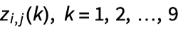 be the element
 ![]() of vector
of vector ![]() . When
. When  , then
 ![]() holds the number
holds the number ![]() . Each
. Each ![]() contains only one number, so
contains only one number, so ![]() can contain only one nonzero element, i.e.
can contain only one nonzero element, i.e. 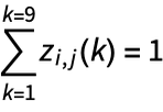 :
:

✕
Clear[z];
squareConstraints =
  Table[{Total[z[i, j]] == 1,
    0 \[VectorLessEqual] z[i, j] \[VectorLessEqual] 1,
    z[i, j] \[Element] Vectors[9, Integers]}, {i, 9}, {j, 9}];
|
Applying the first sudoku rule, each row must contain all the numbers, i.e. 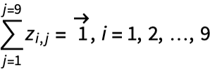 , where
 ![]() is a nine-dimensional vector of ones:
is a nine-dimensional vector of ones:
|
✕
onesVector = ConstantArray[1, 9];
rowConstraints = Table[Sum[z[i, j], {j, 9}] == onesVector, {i, 9}];
|
The second rule says that each column must contain all the numbers, i.e. 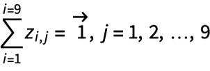 :
:
|
✕
columnConstraints = Table[Sum[z[i, j], {i, 9}] == onesVector, {j, 9}];
|
The third rule says that each 3×3 block must contain all the numbers, i.e.  :
:
|
✕
blockConstraints =
  Table[Sum[z[i + m, j + n], {m, 3}, {n, 3}] ==
    onesVector, {i, {0, 3, 6}}, {j, {0, 3, 6}}];
|
Collectively, these make the sudoku constraints for any puzzle:
|
✕
sudokuConstraints = {squareConstraints, rowConstraints,
   columnConstraints, blockConstraints};
|
Collect all the variables:
|
✕
vars = Flatten[Table[z[i, j], {i, 9}, {j, 9}]];
|
Convert the known values into constraints. If element ![]() holds number
holds number ![]() , then
, then  :
:

✕
knownConstraints =
  MapThread[
   Indexed[z @@ #1, #2] == 1 &, {initialSudokuBoard[
     "NonzeroPositions"], initialSudokuBoard["NonzeroValues"]}];
|
LinearOptimization is typically used to minimize a linear objective subject to a set of linear constraints. In this case, the objective is 0 since there is no objective other than interest in a feasible solution:

✕
res = LinearOptimization[0, {sudokuConstraints, knownConstraints},
   vars];
Short[res, 3]
|
To know which number goes into which position, the information must be extracted from the vectors ![]() . This is easily done as:
. This is easily done as:

✕
Short[pos =
  MapThread[List @@ #1 -> Range[9].#2 &, {vars, vars /. res}], 4]
|
Visualize the result by converting the previous output into a SparseArray:

✕
ResourceFunction["DisplaySudokuPuzzle"][SparseArray[pos]] |
As you can see, putting the problem together and solving it took 6–7 lines of code. This procedure has been placed as a ResourceFunction called SolveSudokuPuzzle that users can call to solve a sudoku puzzle:

✕
ResourceFunction["SolveSudokuPuzzle"][initialSudokuBoard] |
This function has been made quite general and has the capacity to solve sudoku puzzles of arbitrary size. The solver also accepts negative numbers being present on the board. If a negative number exists, then the solver tries to solve the puzzle with the assumption that the number at that position cannot exist.
Generating a Sudoku Puzzle
The strategy we will use to generate a sudoku puzzle is to start with a full board. From this, an element will be randomly selected and the number that lies at that element will be removed. We will then enforce a condition that the number we removed from that element cannot lie at that element. If the solver comes back with a solution despite the additional condition, it means that the number at that position is not unique and cannot leave the board. If the solver comes back with a failed result, then that number at that position is unique and can be removed.
To implement this strategy, there needs to be a way to generate a full random sudoku board. There are several approaches that one can use to generate a full sudoku board. One approach would be to randomly specify the diagonal entries of the sudoku board and allow the solver to generate a puzzle for us:

✕
fullSudokuPuzzle = ResourceFunction["SolveSudokuPuzzle"][ SparseArray@DiagonalMatrix[RandomSample[Range[9]]]]; ResourceFunction["DisplaySudokuPuzzle"][fullSudokuPuzzle] |
This will generate three hundred thousand possible puzzles. One advantage our solver has is that we can also specify that certain numbers cannot be present at a particular position. This is done by making that number negative at that position. Taking advantage of this feature, over one hundred million puzzles can be generated by modifying the procedure:

✕
initialPuzzle = SparseArray@DiagonalMatrix[
    RandomSample[Range[9]]*RandomChoice[{1, -1}, 9]];
refSudokuMat = ResourceFunction["SolveSudokuPuzzle"][initialPuzzle];
ResourceFunction["DisplaySudokuPuzzle"][refSudokuMat]
|
Of course, this is still a very small fraction of the total possible boards, but it is a start.
Now that we have a full board, let us assume that we want to keep only 50 elements from the board. The iterative code would be:

✕
minElementsToKeep = 50;
sudokuElements = RandomSample[Thread[
    refSudokuMat["NonzeroPositions"] ->
     refSudokuMat["NonzeroValues"]]];
n = 81; i = 1;
While[Length[sudokuElements] > minElementsToKeep && i < n,
  newElements = sudokuElements;
  newElements[[i, 2]] *= -1;
  res = ResourceFunction["SolveSudokuPuzzle"][
    SparseArray[newElements, {9, 9}]];
  If[res === $Failed, sudokuElements = Delete[sudokuElements, i]; n--,
    i++];];
|
Note the extra condition, where numbers that cannot appear at certain positions are removed by making those numbers negative. We can now display our freshly minted sudoku puzzle:

✕
sudokuPuzzle = SparseArray[sudokuElements, {9, 9}, _];
ResourceFunction["DisplaySudokuPuzzle"][sudokuPuzzle]
|
It’s possible to double-check that the puzzle can be solved and that the result we get back is the same as the reference sudoku we started with:

✕
ResourceFunction["DisplaySudokuPuzzle"][#] & /@ {refSudokuMat,
  ResourceFunction["SolveSudokuPuzzle"][sudokuPuzzle]}
|
Notice that the solved puzzle recovered the reference puzzle.
A ResourceFunction called GenerateSudokuPuzzle has been developed for the user’s convenience that will generate sudoku puzzles of different sizes and determine how many elements need to be exposed:

✕
{fullBoard, sudokuPuzzle} =
 ResourceFunction["GenerateSudokuPuzzle"][3, 0.4]
|

✕
ResourceFunction["DisplaySudokuPuzzle"][#] & /@ {fullBoard,
  sudokuPuzzle}
|
Due to the general nature of the function, sudoku boards can be generated in different sizes. Here is a 4×4 board:

✕
{fullBoard, sudokuPuzzle} =
  ResourceFunction["GenerateSudokuPuzzle"][2, 0.5];
ResourceFunction["DisplaySudokuPuzzle"][#] & /@ {fullBoard,
  sudokuPuzzle}
|
Next is a 16×16 board. The computation time to generate boards increases considerably with size because there are now 256 binary vectors of length 16 (as opposed to 81 vectors of length 9 for the 9×9 case). The following one took about 30 seconds to generate (but will change for every run):

✕
{fullBoard, sudokuPuzzle} =
  ResourceFunction["GenerateSudokuPuzzle"][4, 0.6];
ResourceFunction["DisplaySudokuPuzzle"][#] & /@ {fullBoard,
  sudokuPuzzle}
|
I will be honest: I did not have the courage to solve this sudoku puzzle. I would love to hear from you if you have attempted to solve one of these large puzzles!
Determining Difficulty Levels
The avid player will probably ask the next obvious question: “What is the difficulty level of the previous puzzle?” This is a tricky question to answer, and I believe it is subjective. However, we can attempt to rank a generated puzzle between 1 and 10, with 1 being easy and 10 being very hard, by looking at how many positions in the board can have their elements uniquely identified by using the three rules and gradually filling the board till no unique elements are present.
So, for a sudoku puzzle with 40% of elements exposed, the difficulty level will be:

✕
{fullBoard, sudokuPuzzle} =
  ResourceFunction["GenerateSudokuPuzzle"][3, 0.4];
ResourceFunction["EstimateSudokuDifficultyLevel"][sudokuPuzzle]
|
You could generate a puzzle by allowing the puzzle generator to return its hardest possible puzzle by specifying the number of exposed elements to be 0. Of course, that will not be possible, so the generator will return its best puzzle that can be solved uniquely:

✕
{fullBoard, sudokuPuzzle} =
  ResourceFunction["GenerateSudokuPuzzle"][3, 0.];
ResourceFunction["EstimateSudokuDifficultyLevel"][sudokuPuzzle]
|
Of course, every run will yield a different number and puzzle. This is the hard puzzle that the generator returned:

✕
ResourceFunction["DisplaySudokuPuzzle"][sudokuPuzzle] |
Solving Killer Sudoku
The killer sudoku game is a variant of the original. It follows the same three rules of the original game, but instead of having numbers specified at certain positions, the player is provided with a board that looks like this:

Each color group is called a “cage,” and a number is provided for each cage. This number represents the sum of all the numbers in that cage. For example, the top-left cage contains the number 26 and consists of four red squares. This means that the total of the numbers in those four red squares must equal 26.
Within our framework, this is actually remarkably easy to do. The trick in solving the killer sudoku puzzle using LinearOptimization is to associate each of the binary vectors ![]() with another variable
with another variable ![]() that actually contains the number at that position. This is done by adding the following set of constraints in addition to the sudoku solver constraints:
that actually contains the number at that position. This is done by adding the following set of constraints in addition to the sudoku solver constraints:

✕
Short[Table[Indexed[y, {i, j}] == Range[9].z[i, j], {i, 9}, {j, 9}],
  2]
|
There is a ResourceFunction called SolveKillerSudokuPuzzle that incorporates this additional constraint and solves the provided puzzle.
Generating a Killer Sudoku Board
Of course, there still needs to be a way to create the killer sudoku board. My approach was to generate random Tetris block–like patterns and then use MorphologicalComponents to extract the various blocks (I am eager to hear from readers about their creative approaches to generating a killer sudoku puzzle). The approach I outlined lives as a ResourceFunction called GenerateKillerSudokuPuzzle and allows us to generate the required information for a killer sudoku puzzle:

✕
Short[{refSudokuBoard, {cagePos, cageVals}} =
  ResourceFunction["GenerateKillerSudokuPuzzle"][], 4]
|
It would help to visualize this puzzle, and that can be done using DisplayKillerSudokuPuzzle:

✕
ResourceFunction["DisplayKillerSudokuPuzzle"][cagePos, cageVals] |
I should point out that generating the killer sudoku puzzle is actually much easier and cheaper to generate than the traditional sudoku puzzle because there are no elements to remove. This puzzle is generated from the following reference sudoku board:

✕
ResourceFunction["DisplaySudokuPuzzle"][refSudokuBoard] |
You can manually check that the puzzle is valid by adding the numbers in the cages. Our killer sudoku puzzle can now be solved:

✕
solvedPuzzle = ResourceFunction["SolveKillerSudokuPuzzle"][cagePos, cageVals] |
During experimentation, I found that sometimes the integer optimization problem is solved within a few seconds, and sometimes it takes over 30 seconds. So, it is difficult to give a good estimate of how quickly the problem can be solved. Here is the result for this particular case:

✕
ResourceFunction["DisplaySudokuPuzzle"][solvedPuzzle] |
I have also noticed that sometimes the solved puzzle will not match the reference sudoku board. This, in my opinion, is completely fine. In my experience, the larger the cage size, the more flexibility the solver has to get a feasible solution, and the numbers, therefore, can move around. Smaller cages, on the other hand, make the problem more restrictive.
Additional Optimization Tools
I hope I have provided you a brief glimpse into the world of optimization, especially (mixed) integer optimization, and how the optimization framework can be used to solve some fun problems. There are plenty of application examples that you can find in the documentation pages of LinearOptimization, QuadraticOptimization, SecondOrderConeOptimization, SemidefiniteOptimization and ConicOptimization.
You will surely have fun playing and creating your own killer sudoku games. I tried solving a hard one from the web, and after an hour of yelling at the paper, I realized it is just easier for the computer to do it, and, well, here we are. Feel free to share your best puzzles in the comments below, or join the conversation on Wolfram Community.
| Get full access to the latest Wolfram Language functionality with a Mathematica 12.1 or Wolfram|One trial. |

My brother suggested I might like this blog. He was entirely right.
This post actually made my day. You can not imagine just how much time I had spent for this information! Thanks!