Exploring the Enigmatic Star, Eta Carinae
One of the most enigmatic stars in our galaxy is η Carinae (Eta Carinae). However, in its first recorded observation several hundred years ago, Eta Carinae was a star of little note. Since then, it has become a source of astronomical interest due to dramatic brightness variations, which at one time made it the second-brightest star in the sky. In this post, we’ll investigate the star using the Wolfram Language and the Wolfram Function Repository to discover why it’s changed in such a relatively short period of time, both in its appearance and in our interest in it.
Discovery and Naming
Being a star only observable in the Southern Hemisphere, its discovery didn’t originate in antiquity. The first official record of Eta Carinae came from Edmund Halley, of Halley’s Comet fame, in 1677 when he mentioned the star in a new constellation of his own creation called Robur Carolinum. At that time, the modern constellations had not yet been standardized, and the star system was described as being in the large, ancient Greek constellation of Argo Navis (the ship). In the second century, Ptolemy detailed specific stars within the constellation, portions of which appear to skirt the southern skies about the Mediterranean Ocean as observed from Greece.
Johannes Bayer’s system for cataloging stars labeled the brightest star in a constellation using the Greek letter α (alpha), the second brightest β (beta) and so on. Since this newly mentioned star was the seventh brightest in Argo Navis, it earned various labels such as Eta Roboris Caroli, Eta Argus or Eta Navis. Argo Navis was eventually broken up into three official constellations, Carina (the keel), Puppis (the poop deck) and Vela (the sails) due to the original constellation’s large size. Its old name slowly fell out of favor until, in 1930, the International Astronomical Union (IAU) officially defined the modern 88 constellations. Because the star system in question fell into the Carina portion of the old constellation, it became known as η (Eta) Carinae.
We can pull in data from Wolfram|Alpha to visualize some star charts showing the modern constellations of Vela and Puppis, which are the northernmost parts of the obsolete constellation Argo Navis, skirting above the southern horizon as observed from Athens, Greece, in early spring. Some of the bright stars in those constellations are labeled. The modern constellation of Carina is below the horizon.
 Engage with the code in this post by downloading the Wolfram Notebook

✕
GraphicsGrid[{{WolframAlpha[
    "Vela star chart Athens, Greece April 1, 9 PM Eastern European \
Time", {{"ConstellationChartPod:ConstellationData", 1}, "Image"}],
   WolframAlpha[
    "Puppis star chart Athens, Greece April 1, 9 PM Eastern European \
Time", {{"ConstellationChartPod:ConstellationData", 1}, "Image"}]}},
 ImageSize -> 525]
|
The modern constellation of Carina can be seen from the Southern Hemisphere.

✕
Entity["Constellation", "Carina"][ EntityProperty["Constellation", "ConstellationGraphic"]] |
Eta Carinae is best observed in late April—during autumn in the Southern Hemisphere—shown here as it appears from Johannesburg, South Africa.

✕
WolframAlpha["Eta Carinae star chart Johannesburg April 30, 10 PM Eastern European Time", {{"SkyMap:StarData", 1}, "Image"}]
|
Observations
Eta Carinae is likely a member of the Trumpler 16 star cluster, which is composed of a number of the most massive stars known. The star cluster itself is embedded in the larger Carina Nebula. Eta Carinae has been widely accepted to lie at a distance of 7,800 ±330 light years. Recent measurements by the Gaia mission indicated a possibility that it lies even further than previously thought, but these measurements were made using other stars in Trumpler 16 that were not obscured by nebulosity. Methods to determine the distance based on aspects of the Homunculus Nebula support the earlier value more.
Variations in Brightness and the Great Eruption
The American Association of Variable Star Observers (AAVSO) maintains a large collection of variable star data, including light curves. This data can be requested via a form and then returned in a variety of formats, including comma‐separated value (CSV) files.
|
✕
SetDirectory[NotebookDirectory[]]; |
|
✕
aavsoraw = Import["aavsodata_5e3fa24cbf211.txt", "CSV"]; |

✕
properties = aavsoraw[[1]] |
|
✕
lightcurve = {FromJulianDate[#[[1]]], #[[2]]} & /@ (Most /@
     Select[aavsoraw[[2 ;;]][[All, {1, 2, 5}]], #[[3]] === "Vis." &]);
|

✕
DateListPlot[lightcurve, Sequence[
 ScalingFunctions -> {None, "Reverse"}, PlotTheme -> "Detailed",
  PlotRange -> All, ImageSize -> 525]]
|
This data is extremely useful for showing past behavior of the Eta Carinae star system, behavior that shows why Eta Carinae is one of the most enigmatic star systems in our galaxy. For about one hundred years after its discovery, it was just a typical star with an apparent magnitude of roughly 3.3, which made it slightly fainter than the well-known star Albireo in the constellation Cygnus—but as this is not one of the brightest stars in the sky, nothing drew special attention to it at the time. This began to change in 1827 when it was observed to have brightened to first magnitude, putting it on par with well-known bright stars like Antares, Spica and Capella. Then, on December 16, 1837, astronomer Sir John Frederick William Herschel (son of William Herschel), observing from a trip to South Africa, recorded that it had brightened to slightly outshine Rigel, which has an apparent magnitude of about .18. This began an event referred to as the Great Eruption. At its peak brightness, in 1845, it approached a magnitude of –1, making it the second-brightest star in the sky besides the Sun, just behind Sirius. After this event, it began to steadily dim, eventually far below its original brightness. Then, in 1887, there was another brief, but less intense, brightening before fading then resumed, reaching a minimum around eighth magnitude. Then, in 1953, the star was observed to be steadily increasing in brightness with regular variation, leading to today. In 1996 the regular variations were discovered and later found to have a 5.54-year period.
With such odd behavior, we needed a better view of Eta Carinae to give us some direction. In 1995, the Hubble Space Telescope imaged Eta Carinae and this is what it saw (along with a new version taken in 2019):

✕
GraphicsGrid[{{Import[
    "https://upload.wikimedia.org/wikipedia/commons/f/fc/Eta_Carinae.\
jpg"], Import[
    "https://cdn.spacetelescope.org/archives/images/screen/heic1912a.\
jpg"]}}, Sequence[ImageSize -> 525, Spacings -> 0]]
|
Left image: Jon Morse (University of Colorado) and NASA . Right image: NASA, ESA, N. Smith (University of Arizona, Tucson) and J. Morse (BoldlyGo Institute, New York)
These images were taken to highlight ultraviolet wavelengths. The more recent image shows magnesium‐rich (Mg II) regions in blue and nitrogen‐rich (N II) areas in red. The images look almost like something you would see in a modern science fiction movie with digital special effects. It looks like something blew up and we are staring at the resulting fireball! This glowing gas surrounding Eta Carinae is known as the Homunculus Nebula. This nebula almost totally obscures our view of the star from Earth, making it very difficult to obtain detailed information about the things going on inside. It’s estimated that the Homunculus Nebula may contains tens of solar masses, perhaps as many as 40. It’s hard to imagine an eruption powerful enough to shed that much mass.
Spectral Classification
For stars, classification can often be summarized using the spectral class or spectral type. For example, the Sun is a G2V star.
![Entity["Star", "Sun"]["SpectralClass"]](https://content.wolfram.com/sites/39/2020/03/1jb0302img10.png "Entity[\"Star\", \"Sun\"][\"SpectralClass\"]")
✕
Entity["Star", "Sun"]["SpectralClass"] |
The spectral class encodes a variety of information, including temperature and often luminosity, or the kind of star. For the Sun, G2 corresponds to a G-class star with subtype 2; along with the Roman numeral V, this means that it corresponds to a 5,800 K main sequence star with a luminosity approximately equivalent to the Sun.
![ResourceFunction["StellarSpectralClassData"]](https://content.wolfram.com/sites/39/2020/03/1jb0302img11.png "ResourceFunction[\"StellarSpectralClassData\"]")
✕
ResourceFunction[
  "StellarSpectralClassData"]["G2V", {"EffectiveTemperature",
  "StarType", "Luminosity"}]
|
Cooler stars use different letters, like M. These spectral class strings can also include additional annotations:
![ResourceFunction["StellarSpectralClassData"]["M6Ve",](https://content.wolfram.com/sites/39/2020/03/1jb0302img12.png "ResourceFunction[\"StellarSpectralClassData\"][\"M6Ve\",")
✕
ResourceFunction[
  "StellarSpectralClassData"]["M6Ve", {"EffectiveTemperature",
  "StarType", "Luminosity", "Peculiarities"}]
|
Stars can also be hotter and larger:
![ResourceFunction["StellarSpectralClassData"]["F8III",](https://content.wolfram.com/sites/39/2020/03/1jb0302img13.png "ResourceFunction[\"StellarSpectralClassData\"][\"F8III\",")
✕
ResourceFunction[
  "StellarSpectralClassData"]["F8III", {"EffectiveTemperature",
  "StarType", "Luminosity"}]
|
So what is the spectral class of Eta Carinae?
![Entity["Star", "EtaCarinae"]["SpectralClass"]](https://content.wolfram.com/sites/39/2020/03/1jb0302img14.png "Entity[\"Star\", \"EtaCarinae\"][\"SpectralClass\"]")
✕
Entity["Star", "EtaCarinae"]["SpectralClass"] |
I’ve combed the literature trying to find a reliable source that says more about this star than this vague result. About the best I can find is the following, which doesn’t say much more.
![ResourceFunction["StellarSpectralClassData"]["OBepec",](https://content.wolfram.com/sites/39/2020/03/1jb0302img15.png "ResourceFunction[\"StellarSpectralClassData\"][\"OBepec\",")
✕
ResourceFunction[
  "StellarSpectralClassData"]["OBepec", {"EffectiveTemperature",
  "StarType", "Luminosity", "Peculiarities"}]
|
The temperature class portion of the spectral class string can typically range over the letters O, B, A, F, G, K and M, with more recent additional letters to cover faint brown dwarfs: L, T and Y. Within this range, O stars are the hottest and Y are the coolest. Since “OBepec” mentions “OB,” we can at least infer that there are characteristics of O or B stars, but there is no temperature subclass to allow us to quantify a temperature, nor is there a Roman numeral to indicate if we are dealing with a dwarf, giant or supergiant. All we can infer is that it’s “hot” and shows emission lines in the spectrum. How hot? Without more information, it’s hard to be sure. We can provide some broad ranges if we assume full temperature and luminosity class specifications. The coolest B stars are B9 dwarfs, and the hottest known O stars are near O3 (for now we’ll just assume a main sequence dwarf, luminosity class V).
![ResourceFunction["StellarSpectralClassData"][{"B9V", "O3V"}](https://content.wolfram.com/sites/39/2020/03/1jb0302img16.png "ResourceFunction[\"StellarSpectralClassData\"][{\"B9V\", \"O3V\"}")
✕
ResourceFunction["StellarSpectralClassData"][{"B9V",
  "O3V"}, "EffectiveTemperature"]
|
So it appears we are talking temperatures that range anywhere from 11,000 K to 41,000 K, which is a very wide range, so all we can say is that we are looking at much hotter temperatures than the Sun’s 5,770 K.
Line Profiles
From the literature, the spectrum of Eta Carinae shows a number of features that can infer properties of what is inside the nebula. There are many emission lines seen on top of a continuum spectrum, along with some peculiarities. Some of the emission lines observed come from doubly ionized neon, iron and argon. We can obtain some of the known lines using SpectralLineData to obtain about 247 lines to simulate.

✕
lines = Join[
   SpectralLineData[
    EntityClass[
     "AtomicLine", {"Neon", 3}], {Quantity[350, "Nanometers"],
     Quantity[750, "Nanometers"]}],
   SpectralLineData[
    EntityClass[
     "AtomicLine", {"Iron", 3}], {Quantity[350, "Nanometers"],
     Quantity[750, "Nanometers"]}],
   SpectralLineData[
    EntityClass[
     "AtomicLine", {"Argon", 3}], {Quantity[350, "Nanometers"],
     Quantity[750, "Nanometers"]}]];
|
|
✕
linevalues = QuantityMagnitude[SpectralLineData[lines, "Wavelength"], "Nanometers"]; |

✕
lineintensity = SpectralLineData[lines, "Intensity"]; Length[linevalues] |
The spectral lines observed in the spectrum of Eta Carinae don’t follow a Gaussian distribution, as you might expect, but instead follow a profile that has an absorption peak preceding the emission peak.
|
✕
pm[x_] := 7 x Exp[(-If[x > 0, 8 x, -16 x])/2] |

✕
Plot[pm[x], {x, -1, 1}]
|
We can offset each line by its wavelength, λ, and perform some scaling and cropping to get the effect needed.

✕
lineprofile[\[Lambda]_, x_, nlines_] :=
 With[{center = x - \[Lambda] + .07},
  Piecewise[
   {
    {pm[center] + .45/nlines, -.4 - center <= center <= .6 - center},
    {.15/nlines, True}
    }
   ]
  ]
|
|
✕
lineprofile[lst_List, x_] := Plus @@ (lineprofile[#, x, Length[lst]] & /@ lst) |
Plotting all of the requested lines in the visible spectrum shows a fair number of lines to examine:

✕
DensityPlot[x, {x, 400, 700}, {y, 0, 1},
 ColorFunction -> (Darker[ColorData["VisibleSpectrum", #],
     1 - 3 Total[lineprofile[linevalues, #]]] &),
 ColorFunctionScaling -> False, AspectRatio -> .1,
 Background -> Black, FrameStyle -> White,
 FrameTicks -> {True, False}, FrameTicksStyle -> White,
 PlotPoints -> {2000, 3}, PlotRangePadding -> None, ImageSize -> 650]
|
Zooming into the blue part of the spectrum, we can see some of the individual lines and that there is a dark absorption feature on the blue side of each line:

✕
DensityPlot[x, {x, 450, 500}, {y, 0, 1},
 ColorFunction -> (Darker[ColorData["VisibleSpectrum", #],
     1 - 3 Total[lineprofile[linevalues, #]]] &),
 ColorFunctionScaling -> False, AspectRatio -> .1,
 Background -> Black, FrameStyle -> White,
 FrameTicks -> {True, False}, FrameTicksStyle -> White,
 PlotPoints -> {2000, 3}, PlotRangePadding -> None, ImageSize -> 650]
|
Stars like the Sun are typically seen as a continuum with absorption lines overlaid. Emission lines are typical of diffuse, ionized gas. In addition, the spectrum of Eta Carinae exhibits shallow absorption features, just to the blue side of each emission line in the previous image.
Although the inner regions of the Homunculus Nebula are obscured from view, the composition of the ejecta from the Great Eruption seems to suggest a mix of approximately 60% hydrogen and 40% helium, with traces of nitrogen being detected in the neighborhood of 10 times what is seen in the solar spectrum.
More Peculiarities
Eta Carinae is the only known instance of naturally formed UV lasers. Lyman-alpha emission, originating in blobs of gas within the system, is able to pump some ionized iron ions into pseudo‐metastable states and results in stimulated emission of radiation within the UV range.
As early as 1972, x‐rays were detected from Eta Carinae from rocket‐based observations. There are a number of different x‐ray sources found at Eta Carinae, ranging from soft to hard. Soft x‐rays are found in various locations within the surrounding nebulosity. Hard x‐rays appear to originate closer to the star itself. Every 5.54 years, the x‐ray spectrum appears to rise, collapse and disappear for about three months, and then recover.
Nuclear Reactions
So what else can we look at to try to come up with some idea of what is going on at Eta Carinae? We can investigate nuclear reactions. Stars that are the temperature of our Sun undergo fusion in their cores via the proton‐proton chain, where hydrogen is converted to helium with deuterium and helium-3 as intermediate reactants. This is the most dominant reaction in the Sun. With lower frequency, other helium-generating reactions happen in the Sun that involve beryllium, lithium and boron.

✕
GraphicsGrid[{{Graph[{
     {1, Entity["Isotope", "Hydrogen1"]} -> {2,
       Entity["Isotope", "Hydrogen1"]}, {2,
       Entity["Isotope", "Hydrogen1"]} -> {1,
       Entity["Isotope", "Hydrogen2"]}, {3,
       Entity["Isotope", "Hydrogen1"]} -> {1,
       Entity["Isotope", "Hydrogen2"]}, {1,
       Entity["Isotope", "Hydrogen2"]} -> {1,
       Entity["Isotope", "Helium3"]}, {4,
       Entity["Isotope", "Hydrogen1"]} -> {5,
       Entity["Isotope", "Hydrogen1"]}, {5,
       Entity["Isotope", "Hydrogen1"]} -> {2,
       Entity["Isotope", "Hydrogen2"]}, {6,
       Entity["Isotope", "Hydrogen1"]} -> {2,
       Entity["Isotope", "Hydrogen2"]}, {2,
       Entity["Isotope", "Hydrogen2"]} -> {2,
       Entity["Isotope", "Helium3"]}, {1,
       Entity["Isotope", "Helium3"]} -> {2,
       Entity["Isotope", "Helium3"]}, {2,
       Entity["Isotope", "Helium3"]} -> {1,
       Entity["Isotope", "Helium4"]}, {1,
       Entity["Isotope", "Helium4"]} -> {7,
       Entity["Isotope", "Hydrogen1"]}, {1,
       Entity["Isotope", "Helium4"]} -> {8,
       Entity["Isotope", "Hydrogen1"]}
     }, VertexLabels -> {{
Blank[],
Pattern[e,
Blank[Entity]]} :> Style[
e["FullSymbol"], 12]}],
   Graph[{{1, Entity["Isotope", "Helium3"]} -> {1,
       Entity["Isotope", "Helium4"]}, {1,
       Entity["Isotope", "Helium4"]} -> {1,
       Entity["Isotope", "Beryllium7"]}, {1,
       Entity["Isotope", "Beryllium7"]} -> {1,
       Entity["Isotope", "Lithium7"]}, {1,
       Entity["Isotope", "Hydrogen1"]} -> {1,
       Entity["Isotope", "Lithium7"]}, {1,
       Entity["Isotope", "Lithium7"]} -> {2,
       Entity["Isotope", "Helium4"]}, {1,
       Entity["Isotope", "Lithium7"]} -> {3,
       Entity["Isotope", "Helium4"]}},
    VertexLabels -> {{
Blank[],
Pattern[e,
Blank[Entity]]} :> Style[
e["FullSymbol"], 12]}],
   Graph[{
     {1, Entity["Isotope", "Helium3"]} -> {1,
       Entity["Isotope", "Helium4"]}, {1,
       Entity["Isotope", "Helium4"]} -> {1,
       Entity["Isotope", "Beryllium7"]}, {1,
       Entity["Isotope", "Hydrogen1"]} -> {1,
       Entity["Isotope", "Beryllium7"]}, {1,
       Entity["Isotope", "Beryllium7"]} -> {1,
       Entity["Isotope", "Boron8"]}, {1,
       Entity["Isotope", "Boron8"]} -> {1,
       Entity["Isotope", "Beryllium8"]}, {1,
       Entity["Isotope", "Beryllium8"]} -> {2,
       Entity["Isotope", "Helium4"]}, {1,
       Entity["Isotope", "Beryllium8"]} -> {3,
       Entity["Isotope", "Helium4"]}
     },
    VertexLabels -> {{
Blank[],
Pattern[e,
Blank[Entity]]} :> Style[
e["FullSymbol"], 12]}]}}, Sequence[ImageSize -> 600, Spacings -> 0]]
|
As the core of a star gets hotter, other reactions become more probable, including one called the carbon–nitrogen–oxygen (CNO) cycle, which is dominant at core temperatures exceeding 17 million Kelvins. The Sun currently only obtains 1.7% of its helium production from the CNO cycle. The CNO cycle uses the trace elements carbon, nitrogen and oxygen as catalysts in the production of helium and results in an enrichment of nitrogen at the sacrifice of the carbon and oxygen. This alters the abundance ratios of these trace elements and deep convection stirs this higher nitrogen ratio toward the surface. So the relatively high levels of nitrogen observed in the ejecta of the Great Eruption could be indicating that the origin of the ejecta came from a star undergoing hydrogen fusion via the CNO cycle. The following graph shows the three primary CNO cycle variants that appear in stars of varying masses and temperatures. Gamma rays, positrons and neutrinos as byproducts are ignored in this graph. There are additional CNO cycles that can occur under particularly energetic environments, like novae and x‐ray bursts, but those are ignored here.

✕
cno1 = With[{isotopes = {Entity["Isotope", "Carbon12"],
      Entity["Isotope", "Nitrogen13"], Entity["Isotope", "Carbon13"],
      Entity["Isotope", "Nitrogen14"], Entity["Isotope", "Oxygen15"],
      Entity["Isotope", "Nitrogen15"], Entity["Isotope", "Carbon12"]}},
   Graph[Join[
     Rule @@@ (Partition[isotopes, 2, 1]), {{1,
        Entity["Isotope", "Hydrogen1"]} ->
       Entity["Isotope", "Carbon12"], {2,
        Entity["Isotope", "Hydrogen1"]} ->
       Entity["Isotope", "Carbon13"], {3,
        Entity["Isotope", "Hydrogen1"]} ->
       Entity["Isotope", "Nitrogen14"], {4,
        Entity["Isotope", "Hydrogen1"]} ->
       Entity["Isotope", "Nitrogen15"],
      Entity["Isotope", "Carbon12"] -> {1,
        Entity["Isotope", "Helium4"]}}],
    VertexLabels -> {Entity["Isotope", "Carbon12"] :> Style[
Grid[{{
Style[12, Smaller], "C"}, {
Style[6, Smaller], SpanFromAbove}},
         Alignment -> {{Right, Center}, {Center}},
         Spacings -> {0, 0}], 10],
      Entity["Isotope", "Nitrogen13"] :> Style[
Grid[{{
Style[13, Smaller], "N"}, {
Style[7, Smaller], SpanFromAbove}},
         Alignment -> {{Right, Center}, {Center}},
         Spacings -> {0, 0}], 10],
      Entity["Isotope", "Carbon13"] :> Style[
Grid[{{
Style[13, Smaller], "C"}, {
Style[6, Smaller], SpanFromAbove}},
         Alignment -> {{Right, Center}, {Center}},
         Spacings -> {0, 0}], 10],
      Entity["Isotope", "Nitrogen14"] :> Style[
Grid[{{
Style[14, Smaller], "N"}, {
Style[7, Smaller], SpanFromAbove}},
         Alignment -> {{Right, Center}, {Center}},
         Spacings -> {0, 0}], 10],
      Entity["Isotope", "Oxygen15"] :> Style[
Grid[{{
Style[15, Smaller], "O"}, {
Style[8, Smaller], SpanFromAbove}},
         Alignment -> {{Right, Center}, {Center}},
         Spacings -> {0, 0}], 10],
      Entity["Isotope", "Nitrogen15"] :> Style[
Grid[{{
Style[15, Smaller], "N"}, {
Style[7, Smaller], SpanFromAbove}},
         Alignment -> {{Right, Center}, {Center}},
         Spacings -> {0, 0}], 10],
      Entity["Isotope", "Carbon12"] :> Style[
Grid[{{
Style[12, Smaller], "C"}, {
Style[6, Smaller], SpanFromAbove}},
         Alignment -> {{Right, Center}, {Center}},
         Spacings -> {0, 0}], 10], {
Blank[],
Pattern[e,
Blank[Entity]]} :> Style[
e["FullSymbol"], 10]}]];
|

✕
cno2 = With[{isotopes = {Entity["Isotope", "Nitrogen15"],
      Entity["Isotope", "Oxygen16"], Entity["Isotope", "Fluorine17"],
      Entity["Isotope", "Oxygen17"], Entity["Isotope", "Nitrogen14"],
      Entity["Isotope", "Oxygen15"], Entity["Isotope", "Nitrogen15"]}},
   Graph[Join[
     Rule @@@ (Partition[isotopes, 2, 1]), {{1,
        Entity["Isotope", "Hydrogen1"]} ->
       Entity["Isotope", "Nitrogen15"], {2,
        Entity["Isotope", "Hydrogen1"]} ->
       Entity["Isotope", "Oxygen16"], {3,
        Entity["Isotope", "Hydrogen1"]} ->
       Entity["Isotope", "Oxygen17"], {4,
        Entity["Isotope", "Hydrogen1"]} ->
       Entity["Isotope", "Nitrogen14"],
      Entity["Isotope", "Nitrogen14"] -> {1,
        Entity["Isotope", "Helium4"]}}],
    VertexLabels -> {Entity["Isotope", "Nitrogen15"] :> Style[
Grid[{{
Style[15, Smaller], "N"}, {
Style[7, Smaller], SpanFromAbove}},
         Alignment -> {{Right, Center}, {Center}},
         Spacings -> {0, 0}], 10],
      Entity["Isotope", "Oxygen16"] :> Style[
Grid[{{
Style[16, Smaller], "O"}, {
Style[8, Smaller], SpanFromAbove}},
         Alignment -> {{Right, Center}, {Center}},
         Spacings -> {0, 0}], 10],
      Entity["Isotope", "Fluorine17"] :> Style[
Grid[{{
Style[17, Smaller], "F"}, {
Style[9, Smaller], SpanFromAbove}},
         Alignment -> {{Right, Center}, {Center}},
         Spacings -> {0, 0}], 10],
      Entity["Isotope", "Oxygen17"] :> Style[
Grid[{{
Style[17, Smaller], "O"}, {
Style[8, Smaller], SpanFromAbove}},
         Alignment -> {{Right, Center}, {Center}},
         Spacings -> {0, 0}], 10],
      Entity["Isotope", "Nitrogen14"] :> Style[
Grid[{{
Style[14, Smaller], "N"}, {
Style[7, Smaller], SpanFromAbove}},
         Alignment -> {{Right, Center}, {Center}},
         Spacings -> {0, 0}], 10],
      Entity["Isotope", "Oxygen15"] :> Style[
Grid[{{
Style[15, Smaller], "O"}, {
Style[8, Smaller], SpanFromAbove}},
         Alignment -> {{Right, Center}, {Center}},
         Spacings -> {0, 0}], 10],
      Entity["Isotope", "Nitrogen15"] :> Style[
Grid[{{
Style[15, Smaller], "N"}, {
Style[7, Smaller], SpanFromAbove}},
         Alignment -> {{Right, Center}, {Center}},
         Spacings -> {0, 0}], 10], {
Blank[],
Pattern[e,
Blank[Entity]]} :> Style[
e["FullSymbol"], 10]}]];
|

✕
cno3 = With[{isotopes = {Entity["Isotope", "Oxygen17"],
      Entity["Isotope", "Fluorine18"], Entity["Isotope", "Oxygen18"],
      Entity["Isotope", "Nitrogen15"], Entity["Isotope", "Oxygen16"],
      Entity["Isotope", "Fluorine17"], Entity["Isotope", "Oxygen17"]}},
   Graph[Join[
     Rule @@@ (Partition[isotopes, 2, 1]), {{1,
        Entity["Isotope", "Hydrogen1"]} ->
       Entity["Isotope", "Oxygen17"], {2,
        Entity["Isotope", "Hydrogen1"]} ->
       Entity["Isotope", "Oxygen18"], {3,
        Entity["Isotope", "Hydrogen1"]} ->
       Entity["Isotope", "Nitrogen15"], {4,
        Entity["Isotope", "Hydrogen1"]} ->
       Entity["Isotope", "Oxygen16"],
      Entity["Isotope", "Nitrogen15"] -> {1,
        Entity["Isotope", "Helium4"]}}],
    VertexLabels -> {Entity["Isotope", "Oxygen17"] :> Style[
Grid[{{
Style[17, Smaller], "O"}, {
Style[8, Smaller], SpanFromAbove}},
         Alignment -> {{Right, Center}, {Center}},
         Spacings -> {0, 0}], 10],
      Entity["Isotope", "Fluorine18"] :> Style[
Grid[{{
Style[18, Smaller], "F"}, {
Style[9, Smaller], SpanFromAbove}},
         Alignment -> {{Right, Center}, {Center}},
         Spacings -> {0, 0}], 10],
      Entity["Isotope", "Oxygen18"] :> Style[
Grid[{{
Style[18, Smaller], "O"}, {
Style[8, Smaller], SpanFromAbove}},
         Alignment -> {{Right, Center}, {Center}},
         Spacings -> {0, 0}], 10],
      Entity["Isotope", "Nitrogen15"] :> Style[
Grid[{{
Style[15, Smaller], "N"}, {
Style[7, Smaller], SpanFromAbove}},
         Alignment -> {{Right, Center}, {Center}},
         Spacings -> {0, 0}], 10],
      Entity["Isotope", "Oxygen16"] :> Style[
Grid[{{
Style[16, Smaller], "O"}, {
Style[8, Smaller], SpanFromAbove}},
         Alignment -> {{Right, Center}, {Center}},
         Spacings -> {0, 0}], 10],
      Entity["Isotope", "Fluorine17"] :> Style[
Grid[{{
Style[17, Smaller], "F"}, {
Style[9, Smaller], SpanFromAbove}},
         Alignment -> {{Right, Center}, {Center}},
         Spacings -> {0, 0}], 10],
      Entity["Isotope", "Oxygen17"] :> Style[
Grid[{{
Style[17, Smaller], "O"}, {
Style[8, Smaller], SpanFromAbove}},
         Alignment -> {{Right, Center}, {Center}},
         Spacings -> {0, 0}], 10], {
Blank[],
Pattern[e,
Blank[Entity]]} :> Style[
e["FullSymbol"], 10]}]];
|

✕
GraphicsGrid[{{cno1, cno2, cno3}}, ImageSize -> 500]
|
Because the Homunculus Nebula seems to show an enrichment of nitrogen compared to solar values, this seems to suggest that the source of the Homunculus Nebula was undergoing the CNO cycle.
Theoretical Explanations
Spectral Lines
As discussed earlier, there are a number of lines seen in the spectrum of the star, many of which come from doubly ionized neon, iron and argon, among other elements. To ionize these elements to this level requires some very high temperatures, supporting the notion that we are dealing with a very hot environment. The ionization levels seen in the spectrum require a source that is at least 37,000 K, which is very hot for a star!
Concerning the strange shape of the observed spectral lines, this is known as a P Cygni profile, named for the star P Cygni, which was the prototype. This observation implies the star is surrounded by an ionized shell of diffuse gas that is expanding outward, creating the emission lines. The blue‐shifted absorption feature is caused by the shell’s absorption of the star’s light along our line of sight. The line‐of‐sight absorption from the shell is blue‐shifted relative to the general emission because it’s only on the side moving toward the Earth.

✕
Graphics[{LightGray, Annulus[{0, 0}, {2, 2.5}],
  Black, {Dashed,
   Line[{{{-.2, 0}, {-.2, -2}}, {{.2, 0}, {.2, -2}}}]},
  Annulus[{0, 0}, {2, 2.5}, {3 Pi/2 - .1, 3 Pi/2 + .1}],
  ColorData["BlackBodySpectrum"][11000],
  Disk[{0, 0}, .2],
  Gray, Arrowheads[.02],
  Arrow@Table[{2.8 {Cos[t], Sin[t]}, 3.1 {Cos[t], Sin[t]}}, {t, 0,
     2 Pi, .1}], Text["To Earth", {0, -3.3}],
  Text["star", {0, 0}, {0, -3}], Text["expanding shell", {0, 1.7}],
  Text["absorption along line of sight", {2.5, -3}],
  Arrow[{{1.2, -3}, {0, -2.6}}]}]
|
Multiple-Star System
In 1996, it was suggested that observed brightness variations had a period, eventually narrowed down to 5.54 years. This suggested the possibility that the variations were caused by a binary star system with an orbital period of 5.54 years. Follow-up spectral observations supported this theory, showing radial velocity variations. X-ray emissions were found to disappear during a relatively brief interval during the predicted time when the stars in the system would be at their closest approach.
Following is an illustration of how the theoretical binary star system could be arranged. Each star has a stellar wind, with the secondary star having a thin and fast wind, while the primary star is nearly obscured by an optically thick and relatively slow wind.

✕
With[{e = .9, a = 15.5, i = -41 Degree},
 With[{b = Sqrt[a^2 - a^2 e^2],
   wind1 = DensityPlot3D[
     Exp[-(x^2 + y^2 + z^2)/2], {x, y, z} \[Element]
      Ball[{0, 0, 0}, 8], Sequence[ColorFunction -> (GrayLevel[
Rescale[#, {0, 1}, {1, 0}]]& ), OpacityFunction -> "Image3D"]]},
  Show[{ParametricPlot3D[{a Cos[t] - (a - a (1 - e)), b Sin[t],
      0}, {t, 0, 2 Pi}, PlotStyle -> Directive[
GrayLevel[0.5],
Thickness[0.002]]],
    Graphics3D[{Gray, Arrowheads[.02],
      Arrow[Table[{a Cos[t - Pi/1.9] - (a - a (1 - e)),
         b Sin[t - Pi/1.9], 0}, {t, 0, 2 Pi, 2 Pi/200}]], RGBColor[
      0.6998692810457516, 0.7757734204793029, 1.],
      Lighting -> {{"Ambient", GrayLevel[.3]}, {"Directional", White,
         ImageScaled[{0, 0, 1}]}}, Sphere[{0, 0, 0}, .279],
      Opacity[.75], RGBColor[
      0.6998692810457516, 0.7757734204793029, 1.], wind1[[1]],
      Opacity[1], RGBColor[
      0.6998692810457516, 0.7757734204793029, 1.],
      Sphere[Table[{a Cos[t] - (a - a (1 - e)), b Sin[t],
         0}, {t, -Pi/2, Pi/2, Pi/10}], .11], , Opacity[.075],
      Sphere[Table[{a Cos[t] - (a - a (1 - e)), b Sin[t],
         0}, {t, -Pi/2, Pi/2, Pi/10}], 1.25], White, Opacity[1],
      Text[\!\(\*
StyleBox["\"\<\[Eta] Carinae A\>\"",
StripOnInput->False,
FontSize->20,
FontWeight->Bold]\), {0, 0, 0}, {0, 7}], Text[\!\(\*
StyleBox["\"\<orbit of \[Eta] Carinae B\>\"",
StripOnInput->False,
FontSize->14,
FontWeight->Bold]\), {-16, -10, 0}, {0, -2}], Text[\!\(\*
StyleBox["\"\<optically thin, fast stellar wind\>\"",
StripOnInput->False,
FontSize->14,
FontWeight->Bold]\), {-10, -10, 0}, {-.2, -2}], Text[\!\(\*
StyleBox["\"\<optically thick stellar wind\>\"",
StripOnInput->False,
FontSize->14,
FontWeight->Bold]\), {-5, 0, 0}, {0, -2}], Black,
      Arrow[{{1, 0, -2}, {0, 0, -.5}}], Red, Arrowheads[.01],
      Arrow[{{-10, -10, 0}, {-10, -8, 0}}],
      Arrow[{{-5, 0, 0}, {-2, 0, 0}}],
      Arrow[{{-16, -10, 0}, {-16, -7.5, 0}}]}]}, Sequence[
   ViewPoint -> {0, (-2) Cos[41 Degree], (-2) Sin[41 Degree]},
    ImageSize -> 650, Background -> GrayLevel[0], Boxed -> False,
    Axes -> False, SphericalRegion -> True,
    ViewAngle -> Rational[1, 8] Pi, ViewVertical -> {-0.3, 0, 1},
    PlotRange -> All]]]]
|
Eta Carinae A is most likely an atypical and extreme luminous blue variable star (LBV) undergoing tremendous mass loss due to its intense stellar wind. Little is known about these types of stars because they are so rare. Eta Carinae B is likely less massive than the primary star, but it may be more evolved. Such a hot star could indicate that it is what is known as a Wolf–Rayet star. Its outer hydrogen envelope has been stripped away, revealing its hotter, helium-rich inner layers. Details of the exact nature of the component stars are difficult to pin down due to surrounding dust, nebulosity and stellar winds, but the primary star may be 120 solar masses, give or take. The secondary is probably in the 30–90 solar mass range. Given that the Homunculus Nebula surrounding the system has tens of solar masses locked up and expanding outward, the original mass of the system must have been extremely large if the remnant component stars still have such high masses.
Based on all the observed evidence and the success of models to reproduce observed phenomena, it’s likely that both stars are massive and that the secondary star is the hotter of the two. As mentioned previously, the primary star appears to be an extreme LBV star, although atypical and more luminous than any other known LBV in our galaxy, so this means it’s likely an early type-B star. The estimated luminosity is millions of times the luminosity of the Sun. On the Hertzsprung–Russell (HR) diagram, this places the primary star near the upper left among the hottest and most luminous stars known, but its exact placement is subject to revision as additional evidence comes in. The secondary is harder to classify, but given its likely smaller radius, even a higher temperature of 37,000 K, making it a rare O‐type star, would place it below Eta Carinae A and slightly to the left using HertzsprungRussellDiagram.
![ResourceFunction["HertzsprungRussellDiagram"]](https://content.wolfram.com/sites/39/2020/03/1jb0302img33.png "ResourceFunction[\"HertzsprungRussellDiagram\"]")
✕
ResourceFunction["HertzsprungRussellDiagram"][ Entity["Star", "EtaCarinae"], ImageSize -> 500] |
Wind-Wind Collision
The origin of the hard x‐ray emission in the Eta Carinae system is likely due to the collision between the stellar winds of the binary star components. As the secondary star approaches periastron (closest approach to the primary star), its fast and thin stellar wind plows through the optically thick and slow-moving stellar wind of the primary star. This creates a bow shock, like a boat moving through water, of superheated gas in a hyperbolic cone region (shown in purple in the image below). The gas in this region can be heated to tens of millions of degrees. As the secondary nears periastron, it goes deeper into the primary star’s stellar wind and becomes obscured from view, causing an eclipse of the x‐ray emission. After the secondary star passes periastron, the x‐rays eventually become visible again before trailing off until the next periastron approach, and the cycle repeats.
Here is a sequence of snapshots of the simulation of the bow shock (purple cone) moving through the primary star’s stellar wind. This is mainly an artistic rendering since the actual orientation of the bow shock would be subject to magnetohydrodynamic effects not considered here. These effects, predicted by supercomputer simulations, have shown that the secondary star’s motion through the thick stellar wind of the primary star carves out a cavity that spirals outward.
First, the stellar wind for both stars can be modified as radially symmetric clouds using DensityPlot3D.

✕
wind1 = DensityPlot3D[
   Exp[-(x^2 + y^2 + z^2)/12], {x, y, z} \[Element]
    Ball[{0, 0, 0}, 8], Sequence[ColorFunction -> (GrayLevel[
Rescale[#, {0, 1}, {1, 0}]]& ), OpacityFunction -> "Image3D"]];
wind2 = DensityPlot3D[
   Exp[-(x^2 + y^2 + z^2)/12], {x, y, z} \[Element]
    Ball[{0, 0, 0}, .9], Sequence[ColorFunction -> (GrayLevel[
Rescale[#, {0, 1}, {0.5, 0}]]& ), OpacityFunction -> "Image3D"]];
|
Next, some fixed constants are defined, including some positions and orbital parameters, as well as the shape and initial orientation of the bow shock.

✕
primarystar = {0, 0, 0};
a = 15.5;
e = .9;
b = Sqrt[a^2 - a^2 e^2];
i = -41 Degree;
ha = 1.5;
hb = 1.5;
hc = 1.5;
dirX = {0, 0, 1};
|
Most of the remainder of the task at hand is to assemble the graphics scene by defining a simulation that is dependent on the phase angle of the secondary star as it orbits the primary star.

✕
simulation[angle_] := Module[{secondarystar, dirZ, dirY},
  secondarystar = {a Cos[angle] - (a - a (1 - e)), b Sin[angle], 0};
  dirZ = Normalize[primarystar - secondarystar];
  dirY = Cross[dirZ, dirX];
  Graphics3D[{
    ParametricPlot3D[{a Cos[t] - (a - a (1 - e)), b Sin[t], 0}, {t, 0,
        2 Pi}, PlotStyle -> Directive[
GrayLevel[0.5],
Thickness[0.002]]][[1]],
    ParametricPlot3D[
      Evaluate[
        secondarystar + ha dirX Sinh[v] Cos[\[Theta]] +
         ha dirY Sinh[v] Sin[\[Theta]] - hb dirZ Cosh[v]] +
       2.5 Normalize[(primarystar - secondarystar)], {\[Theta], 0,
       2 Pi}, {v, 0, -2}, Sequence[
      Mesh -> None, PlotStyle -> Directive[
Specularity[
GrayLevel[1], 50],
RGBColor[0.5, 0, 0.5]], Lighting -> {{"Ambient",
GrayLevel[0.7]}, {"Directional",
GrayLevel[1], 0.9 secondarystar}}]][[1]], RGBColor[
    0.6998692810457516, 0.7757734204793029, 1.],
    Lighting -> {{"Ambient", GrayLevel[0.7`]}, {"Directional", White,
       ImageScaled[{0, 0, 1}]}},
    Sphere[primarystar, .279], Opacity[.2], RGBColor[
    0.6998692810457516, 0.7757734204793029, 1.], wind1[[1]],
    Opacity[1], RGBColor[0.6998692810457516, 0.7757734204793029, 1.],
    Sphere[secondarystar, .11], Opacity[.8], wind2[[1]]}, Sequence[
   ViewPoint -> {0, (-2) Cos[i], 2 Sin[i]},
    ViewVertical -> {-0.7, 0, 1}, Boxed -> False, Axes -> None,
    SphericalRegion -> True, ViewAngle -> Rational[1, 15] Pi,
    PlotRange -> 35, Lighting -> {{"Ambient",
GrayLevel[0.7]}, {"Directional",
GrayLevel[1], primarystar}}, Background -> GrayLevel[0],
    ViewCenter -> {0.35, 0.5, 0.5}]]
  ]
|
Several static snapshots of the simulation can be seen using the following.

✕
GraphicsGrid[
 Partition[simulation /@ {-(\[Pi]/3), -(\[Pi]/9), \[Pi]/9, \[Pi]/3},
  2], ImageSize -> 500]
|
Time can be iterated and the frames exported, and then combined in post‐processing to make an animation:

✕
Do[
 Module[{gr},
  gr = simulation[angle];
  Export[ToString[
     PaddedForm[Rescale[angle, {-Pi/3, Pi/3}, {0, 400}], 3,
      NumberPadding -> "0", NumberSigns -> {"", ""}]] <> ".png", gr];
  ], {angle, -Pi/3, Pi/3, Pi/3/200}]
|
Accretion
Some models of the Eta Carinae system show the possibility that within days of periastron passage, the secondary star may actually accrete matter from blobs formed by the shock zone. Higher-mass models of the secondary star favor more accretion than lower-mass models. A higher mass for the secondary star increases the likelihood that gas will be attracted to it and accumulate on its surface, and so slowly increase the mass of the secondary star with possible secondary effects due to the presence of an accretion disk.
Cause of the Eruptions
To this day, neither the Great Eruption observed in the mid‐1800s nor the other smaller eruptions that have been observed are well understood. A number of theories exist to explain the eruptions, but a lack of detail concerning the inner regions of the system makes it difficult to confirm any one of these theories. Obviously, the high mass and instability that comes along with the system likely had something to do with it. One theory suggests that there may have been a triple star system and the third member merged with one of the other stars, causing an outburst. Another is that mass transfer between the primary and secondary stars caused a nova‐like outburst. A third possibility is that due to the large amount of mass involved in the primary star, gamma rays in the core were energetic enough to spontaneously generate electron-positron pairs in significant number. This last theory would have it that the energy created in the core of the primary star, which normally provides radiation pressure to support the star against gravitational collapse, was converted into matter pairs instead. The production of matter pairs results in a pulsational pair-instability supernova, or “supernova impostor.”
The Future Is Bright
As with any star, the end state is primarily mass-dependent. It is widely accepted that Eta Carinae involves at least one very massive star, and it is very likely it contains two of them. In all cases, the masses of the star or stars involved are well above the threshold needed to result in a supernova explosion at some point in the future. The mysteries of the system make it impossible to say exactly when this might happen, especially since there may already have been one failed attempt at a supernova during the Great Eruption. Hopefully, as time progresses, the Homunculus Nebula will expand enough to allow us to have a clear view of the inner regions, and Eta Carinae will finally reveal its secrets.
| Get full access to the latest Wolfram Language functionality with a Mathematica 12 or Wolfram|One trial. |


Outstanding discussion, analysis, and visualization of the Eta Carinae system, Jeff!
I’m awe of your in-depth research and discussion Jeff. Bravo!