Shattering the Plane with Twelve New Substitution Tilings Using 2, φ, ψ, χ, ρ
 substitution tiling fractal")
Similar Triangle Dissections
Version 12 of the Wolfram Language introduces solvers for geometry problems. The documentation for the new function GeometricScene has a neat example showing the following piece of code, with GeometricAssertion calling for seven similar triangles:
 Engage with the code in this post by downloading the Wolfram Notebook
 substitution tiling")
✕
o=Sequence[Opacity[.9],EdgeForm[Black]];plasticDissection=RandomInstance[GeometricScene[{a,b,c,d,e,f,g},{
a=={1,0},e=={0,0},Line[{a,e,d,c}],
p0==Polygon[{a,b,c}],
p1==Style[Polygon[{b,d,c}],Orange,o],
p2==Style[Polygon[{d,f,e}],Yellow,o],
p3==Style[Polygon[{b,f,d}],Blue,o],
p4==Style[Polygon[{g,f,b}],Green,o],
p5==Style[Polygon[{e,g,f}],Magenta,o],
p6==Style[Polygon[{a,e,g}],Purple,o],
GeometricAssertion[{p0,p1,p2,p3,p4,p5,p6},"Similar"]}],RandomSeeding->28]
|
The coordinates of the point  use the plastic constant
  , the real root of
  .
.

✕
{Chop[c/.plasticDissection["Points"]],N[-Sqrt[{8,12,8}.(ρ^{0,1,2})]]}
|
Combinations of  (rho) build the entire triangle, putting it in the algebraic number field
  . Call this the
  dissection. The length of an edge labeled
  is
is  .
.
 substitution tiling")
✕
dissectionDiagram[SqrtRho,400] |
In the initialization section of the notebook, SqrtRho is defined to be the list consisting of the root, the vertices in terms of that root, the subtriangles and the symbol. The function dissectionDiagram uses these values to draw the triangles with the edge lengths equal to powers of  .
.

✕
SqrtRho |
The Cartesian coordinates can be found with SqrtSpace, defined in the initialization section.

✕
N[SqrtSpace[SqrtRho[[1]],SqrtRho[[2]]]] |
Pisot Numbers
The plastic constant  is the smallest Pisot number, an algebraic integer greater than 1 with conjugate elements in the unit disk. Here are the first four and the ninth Pisot numbers, showing the value as a point outside and the conjugate elements inside.

✕
Text[Grid[Transpose[{Style[TraditionalForm[#],10],Max[N[Norm/@(x/.Solve[#==0])]],
Graphics[{Point[ReIm/@(x/.Solve[#==0])], Circle[{0,0},1],Red,
Disk[{0,0},.05]}, ImageSize-> 95]}&/@{-1-x+x^3,-1-x^3+x^4,-1+x^2-x^3-x^4+x^5,-1-x^2+x^3,-1-x^2-x^4+x^5}],Frame-> All]]
|
The second Pisot number  has a real conjugate element
  (chi), with
  .
.

✕
Grid[{N[#,15],TraditionalForm[MinimalPolynomial[#,x]]}&/@{Root[-1-#1^3+#1^4 &,2], -1/Root[-1-#1^3+#1^4 &,1]}, Frame-> All]
|
Here is the second neat example from the documentation mentioned in the opening paragraph. Decompose a polygon into similar triangles:

✕
RandomInstance[GeometricScene[{a, b, c, d, e, o},
  {Polygon[{a, b, c, d, e}],
   p1 == Style[Triangle[{a, b, o}], Red],
   p2 == Style[Triangle[{b, o, c}], Blue],
   p3 == Style[Triangle[{c, d, o}], Yellow],
   p4 == Style[Triangle[{d, o, e}], Purple],
   p5 == Style[Triangle[{e, o, a}], Orange],
   GeometricAssertion[{p1, p2, p3, p4, p5}, "Similar"] } ], RandomSeeding -> 6]
|
That solution can be extended to nine similar triangles.
 substitution tiling")
✕
o=Sequence[Opacity[.9],EdgeForm[Black]];RandomInstance[GeometricScene[{a,b,c,d,e,f,g,h,i},{
h=={0,0},d=={1,0},p0==Polygon[{d,a,i}],
p1==Style[Polygon[{a,b,f}],Magenta,o ],
p2==Style[Polygon[{b,f,g}],Yellow,o],
p3==Style[Polygon[{f,g,e}],Purple,o],
p4==Style[Polygon[{e,g,h}],Blue,o],
p5==Style[Polygon[{h,c,g}],Cyan,o],
p6==Style[Polygon[{d,h,c}],Red,o],
p7==Style[Polygon[{c,g,b}],Orange,o],
p8==Style[Polygon[{a,e,i}],Green,o],
GeometricAssertion[{p0, p1,p2,p3,p4,p5,p6,p7,p8},"Similar"],
Line[{a,b,c,d}],Line[{a,f,e}],Line[{i,e,h,d}]}],RandomSeeding->85 ]
|
These triangles are built with  ; call this the
  dissection. The length of an edge is
  , where
  is the label on the edge.
 substitution tiling")
✕
dissectionDiagram[SqrtChi, 480] |
The Golden and Supergolden Ratios
Related to  and
and  is the golden ratio, introduced in the book Liber Abaci (1202) by Leonardo Bonacci of Pisa. Early in the book is the Arabic number system.

Later in Liber Abaci is the rabbit problem, leading to what is now called the Fibonacci sequence. The name “Fibonacci” was created in 1838 from “filius Bonacci” or “son of Bonacci.”

This shows the Fibonacci rabbit sequence and its relation to  (phi), the golden ratio.

✕
ϕ=GoldenRatio;
rabbitseq=LinearRecurrence[{1,1},{1,1},120];
Grid[{
{"rabbit sequence",Row[Append[Take[rabbitseq,16],"…"],","]},
{"successive ratios",N[rabbitseq[[-1]]/rabbitseq[[-2]],50]},
{"golden ratio",N[ϕ,50]}
},Frame->All]
|
In 1356, Narayana posed the following question in his book Ganita Kaumudi: “A cow gives birth to a calf every year. In turn, the calf gives birth to another calf when it is three years old. What is the number of progeny produced during twenty years by one cow?”
We can use Mathematica to show the Narayana cow sequence and its relation to  (psi), the supergolden ratio.

✕
ψ=Root[-1-#1^2+#1^3&,1];
cowseq=LinearRecurrence[{1,0,1},{1,2,3},180];
Grid[{
{"cow sequence",Row[Append[Take[cowseq,16],"..."],","]},
{"successive ratios",N[cowseq[[-1]]/cowseq[[-2]],50]},
{"supergolden ratio",N[ψ,50]}
},Frame->All]
|
The ratios of consecutive terms in the Padovan sequence and Perrin sequence both tend to  , as shown in Fibonacci and Padovan Spiral Identities and Padovan’s Spiral Numbers. This shows these two sequences with the rabbit and cow sequences:

✕
padovan=LinearRecurrence[{0,1,1}, {2,2,3}, 15];perrin=LinearRecurrence[{0,1,1}, {2,3,2}, 15];
narayana=LinearRecurrence[{1,0,1},{1,2,3},15];
fibonacci=LinearRecurrence[{1,1},{1,1},15];
Column[{TextGrid[Transpose[{{Padovan,Perrin,Narayana, Fibonacci},
Row[Append[#,"…"],","]&/@{padovan,perrin,narayana, fibonacci}}],Frame-> All],
ListLinePlot[Rest[#]/Most[#]&/@{padovan,perrin,narayana, fibonacci},
 PlotRange->{1,2},GridLines->{{}, {ρ,ψ,ϕ}},ImageSize-> Medium]}]
|
Constructing Geometric Figures
The powers  ,
,  and
and  of the golden ratio are the side lengths of the Kepler right triangle. The golden ratio (or Fibonacci rabbit constant) is the Pisot number
  . By using Pisot numbers
  (the plastic constant),
  ,
,  (the supergolden ratio) or
  , the same process makes a 120° angle, as does
  , the tribonacci constant.

✕
Grid[Partition[niceTriangle/@nice[[{2,11,13,8,14,12}]],2]]
|
Almost all the Platonic and Archimedean solids can be built with the octahedral group acting on  or the icosahedral group acting on
  . Exceptions:
- The snub cube needs a root of
 (tribonacci constant).
 - The snub dodecahedron neets a root of

- The snub icosidodecadodecahedron needs an element of
 (not shown).
This builds the first two snubs with vertex coordinates in the given algebraic number fields.

✕
scroot=Root[-1-#1-#1^2+#1^3&,1];
{scv,scf}=Normal[];  scp=SqrtSpace[scroot, scv];
sdroot=Root[-GoldenRatio-#1-#1^2+#1^3&,1];
{sdv,sdf}=Normal[];sdp=SqrtSpace[sdroot, sdv];
GraphicsRow[{
Graphics3D[{EdgeForm[Thick],Opacity[.9],Polygon[scp[[#]]]&/@scf}, Boxed-> False, ViewAngle-> Pi/9],Graphics3D[{EdgeForm[Thick],Opacity[.9],Polygon[sdp[[#]]]&/@sdf}, Boxed-> False,ViewAngle-> Pi/10]},ImageSize-> 530]
|
If two roots have the same discriminant ( ) they usually belong to the same algebraic number field. Here are two polynomials for the tribonacci constant.

✕
Grid[{TraditionalForm[MinimalPolynomial[#,x]],NumberFieldDiscriminant[#]}&/@{Root[-1-#1-#1^2+#1^3&,1], Root[-2+2#1-2#1^2+#1^3&,1]},Frame-> All]
|
The tribonacci constant is part of an odd series of polynomials tying together Heegner numbers and the j-function in a way that leads to extreme almost integers in multiple ways.

✕
heegnergrid |
The silver ratio  also leads to interesting geometry. If a sheet of A4 paper is folded in half, the rectangles are similar to the original rectangle. The A4 rectangle can be perfectly subdivided into smaller distinct A4 rectangles in many strange ways. The values 2,
  ,
,  and
and  are all involved in dissections of squares and similar rectangles.

✕
Grid[{{A4rect,psirect},{goldenrect, plasrect}}]
|
These dissections can be found in Version 12.

✕
o=Sequence[Opacity[1],EdgeForm[Black]];RandomInstance[GeometricScene[{a,b,c,d,e,f,g, h},{
a=={0,0},d=={0,1},
p01==Polygon[{g,h,a}],p02==Polygon[{a,e,g}],
p11==Style[Polygon[{c,b,a}],Orange,o],
p12==Style[Polygon[{a,d,c}],Orange,o],
p21==Style[Polygon[{c,d,e}],Yellow,o],
p22==Style[Polygon[{e,f,c}],Yellow,o],
p31==Style[Polygon[{h,b,f}],LightBlue,o],
p32==Style[Polygon[{f,g,h}],Blue,o],
GeometricAssertion[{p01,p02,p11,p12,p21,p22,p31,p32},"Similar"]}],RandomSeeding->7]
|
The third root  leads to solutions for the disk-covering problem and the Heilbronn triangle problem.

✕
Row[{Melissen12, Heilbronn12}]
|
Infinite Series Series
Many of the numbers introduced so far can be expressed as infinite series of negative powers of themselves.

✕
seriesgrid |
A 45° right triangle of area 2 can be used to prove the first series by splitting smaller and smaller similar triangles. Or use the infinite similar triangle dissection shown here.

✕
start=SqrtSpace[2,{{{18},{0}},{{-18},{0}},{{9},{63}}/8,{{18},{0}},{{-81},{63}}/32}];
Graphics[{Line[Join[start,Flatten[Table[{(2^a -1)/2^a start[[1]]+(1)/2^a start[[2]],
(2^a -1)/2^a start[[1]]+(1)/2^a start[[5]]},{a,1,7}],1]]] }]
|
The infinite series for  can also be illustrated with an infinite set of similar triangles.

✕
forphi=Normal[List];
Graphics[{EdgeForm[Black],{Lighter[Hue[10.8Area[Polygon[#]]]], Polygon[#],Black,
With[{log=Round[Log[GoldenRatio,Area[Polygon[#]]]]},If[log>-10,Text[log,Mean[#]]]]}&/@forphi}]
|
The infinite series for  can be illustrated with an infinite set of similar Rauzy fractals.

✕
r=Root[-1-#1^2+#1^3&,3];Cow[comp_]:=Map[First,Split[
Flatten[RootReduce[Map[Function[x,x[[1]]+(x[[2]]-x[[1]]){0,-r^5,r^5+1,1}],Partition[comp,2,1,1]]]]]];
 poly2=Table[ReIm[Nest[Cow,N[RootReduce[r^({4,1,3,5}+n){1,1,-1,1}],50],3]],{n,1,30}];fracψ=Graphics[{EdgeForm[{Black}],Gray,Disk[{0,0},.1],
Map[Function[x,{ColorData["BrightBands"][N[Norm[Mean[x]]3]],Polygon[x]}],poly2],Black, Inset[Style[Row[{"ψ =",Underoverscript["∑","n=2", "∞"],Superscript["ψ","-n"]}],20],{-1/3,1/3}]}]
|
The infinite series for  can be illustrated with an infinite set of similar fractals.

✕
ρ=Root[-1-#1+#1^3&,3]; iterations=4;big=ρ^{5,8,6,9,4,7};par=ρ^{6,9,7,10,5,8};
wee=ρ^4{ρ^3,ρ^8,ρ^5,ρ^6(2ρ^2 -1),1,ρ^2 (2ρ^3 -1)};
plastic[comp_]:=Map[First,Split[Flatten[RootReduce[Map[Function[x,
{x[[1,1]]+(x[[1,2]]-x[[1,1]]) {0,ρ^5,1},x[[2,1]]+(x[[2,2]]-x[[2,1]]) {0,1-ρ^5,1}}],Partition[Partition[comp,2,1,1],2]]]]]];
poly=Table[{Hue[Pi n],Polygon[ReIm[Nest[plastic,wee ρ^(n-1),iterations]]]},{n,1,20}];Graphics[{EdgeForm[Black],poly, Inset[Style[Row[{"ρ =",Underoverscript["∑","n=4", "∞"],Superscript["ρ","-n"]}],20],{-5/12,1/3}] }, ImageSize-> 500]
|
Here is that grid of values again.

✕
seriesgrid |
Iterated Dissections
It turns out these “self-summing” infinite series also have unusual self-similar triangle dissections, first hinted at in Wheels of Powered Triangles.

✕
Column[dissectionDiagram[#, 530]&/@{SqrtTwo,SqrtPhi,SqrtPsi,SqrtChi,SqrtRho}]
|
Iterate the dissection; to reduce the chaos, triangles with the same orientation are colored the same. Here are the dissections after 18 steps.

✕
Column[labeledrecursionDiagram[#, 530, 18]&/@{SqrtTwo,SqrtPhi,SqrtPsi,SqrtChi,SqrtRho}]
|
The following pinwheel tiling is not nearly as chaotic. Pinwheel triangles eventually have an infinite number of orientations, but the progress to chaos is slower than the ones shown previously.

✕
recursionDiagram[pinwheel, 530, 22] |
Here’s a portion of the  fractal after 180 steps.
 substitution tiling fractal")
✕
pts=Drop[Append[SqrtSpace[SqrtChi[[1]], SqrtChi[[2]]], SqrtSpace[SqrtChi[[1]], {{7,13,11,9},{9,15,13,11}}/4]],{3}];
tri={{2,9,1},{4,6,3},{5,6,8},{7,6,4},{3,5,6},{8,7,6},{1,3,5},{2,8,7}};
edges=Union[Flatten[Subsets[#,{2}]&/@tri,1]];
bary=ReptileSubstitutionBarycentrics[SqrtChi];
start=GatherBy[Chop[N[pts[[#]]]]&/@tri,Area[Polygon[#]]&];
iterate=SortBy[GatherBy[RecursiveBarycentrics[180,bary, start],Round[10^6Normalize[#[[1]]-Mean[#]]]&],Length[#]&];fractchi = Graphics[{EdgeForm[Black], MapIndexed[
{RGBColor[N[(IntegerDigits[#2[[1]],4,3])/3.1]], Polygon[#]&/@#1}&,iterate]}, ImageSize-> 530]
|
And here is a portion of the plastic fractal after 40 steps.
 substitution tiling fractal")
✕
take=SqrtRho;
pts=ReplacePart[SqrtSpace[take[[1]], take[[2]]],3-> SqrtSpace[take[[1]], {{4,1,-3},{4,7,7}}/4]];;
tri=ReplacePart[take[[3]],1-> {2,3,1}];
bary=ReptileSubstitutionBarycentrics[take];
start=GatherBy[Chop[N[pts[[#]]]]&/@tri,Area[Polygon[#]]&];
iterate=SortBy[GatherBy[RecursiveBarycentrics[40,bary, start],Round[10^6Normalize[#[[1]]-Mean[#]]]&],Length[#]&];Graphics[{EdgeForm[Black], MapIndexed[
{RGBColor[N[(IntegerDigits[#2[[1]],4,3])/3.1]], Polygon[#]&/@#1}&,iterate]}, ImageSize-> 530]
|
By using symmetry within the dissections, it turns out there are twelve substitution tilings with distinct properties.

✕
Grid[Partition[dissectionDiagram[#, 265]&/@
{SqrtTwo,SqrtTwo2,SqrtPhi,SqrtPsi,SqrtChi,SqrtChi2,SqrtChi3,SqrtChi4,SqrtRho,SqrtRho2,SqrtRho3,SqrtRho4},UpTo[2]]]
|
It turns out “neat example” is really true here, leading to twelve new substitution tilings.
|
Mathematica 12 significantly extends the reach of Mathematica and introduces many innovations that give all Mathematica users new levels of power and effectiveness. |

Your dissections with xhi seem wrong:
xhi = 1.22074408460576
xhi^4 = 2.22074408460576 vs xhi + 1 = 2.22074408460576
zeta = sqrt(xhi)
zeta^14 = 4.03991659800193 vs zeta^9 + zeta^5 = 4.10013929506199
zeta^14 = 4.03991659800193 vs zeta^11 + zeta^1 = 4.10013929506199
so the left subtriangle has not edge length zeta^14
The main triangle dimensions in order to be fractal is :
a = zeta^7 + 2*zeta^5 + 2*zeta^3 + zeta
b = zeta^6 + zeta^4 + zeta^2 + 1
c = zeta^6 + zeta^4 + 2*zeta^2 + 1
with
a*zeta^0 = c*zeta^3 = b*zeta^5
Yes, that’s valid. Still a set of similar triangles, but I shouldn’t have rounded the power. I’ve decided to cut up that larger triangle.
oddity in the pinwheel diagram — shouldn’t all the sub-triangles be the same size?
Thanks for the new tilings and thorough writeup.