Centenary of Bohr’s Atomic Theory (1913–2013)
I had intended to write a treatise describing the history of the hydrogen atom over the last 100 years. Unfortunately, my time is running out this year, so I will content myself instead with this much briefer blog post outlining the major events associated with Niels Bohr’s three epochal papers in 1913.
The hydrogen atom has been the most fundamental application at each level in the advancement of quantum theory. It is the only real physical system that can be solved exactly (although some might argue that this is also true for the radiation field, as an assembly of harmonic oscillators).
To set the stage for Bohr’s contributions, we need to recount a couple of items in hydrogen’s “prehistory”. Following the discoveries of Kirchhoff and Bunsen, it was known that the emission spectrum of atomic hydrogen contains four lines in the visible region: a red line at 656.21 nm (15239 cm-1), a blue-green line at 486.07 nm (20573 cm-1), and two violet lines at 434.01 nm (23041 -1) and 410.12 nm (24383 cm-1). The spectrum is obtained in the laboratory by passing a 5000 v electrical discharge through gaseous hydrogen. The hydrogen spectrum is simulated in the following figure:

Johann Jacob Balmer, a Swiss high-school mathematics teacher, found that the wavenumbers (1/λ) of the four spectral lines could be fitted to a simple formula
![]()
After more lines in the infrared and ultraviolet spectrum of hydrogen were found, the Swedish physicist Johannes Rydberg proposed a generalization of Balmer’s formula:
![]()
with n1 = 1, 2, 3, …, n2 = n1 + 1, n1 + 2, … and R ≈ 109678 cm-1 (current experimental value), known as the Rydberg constant. The series of lines beginning with n1 = 2 reduces to Balmer’s formula. This is now known as the Balmer series. The more intense series of lines with n1 = 1, discovered in 1906, lie in the ultraviolet spectrum and are known as the Lyman series. The Lyman-alpha line, with n1 = 1, n2 = 2, at 121.57 nm, is now an important marker in astronomical observations of distant galaxies and quasars. A collection of such lines, from varying environments around a high-redshift quasar, has been called a “Lyman-alpha forest”.
Other atomic species produce characteristic line spectra, which can serve as “fingerprints” to identify the element, particularly in distant stars. But no atom other than hydrogen has a simple relationship for its spectral frequencies, nothing analogous to Rydberg’s formula.
J. J. Thomson discovered in 1897 that electrons were a component of all atoms. For several years thereafter, the prevalent picture of the atom was the “plum pudding model”, in which the negatively charged electrons were pictured as plums embedded throughout a positive sphere—the pudding. If the plum pudding model were correct, alpha particles scattered through a metallic foil should be deflected by, at most, small angles. The positive-charge distribution would then show a diameter of the order of 10-8 cm, the square root of the scattering cross section.
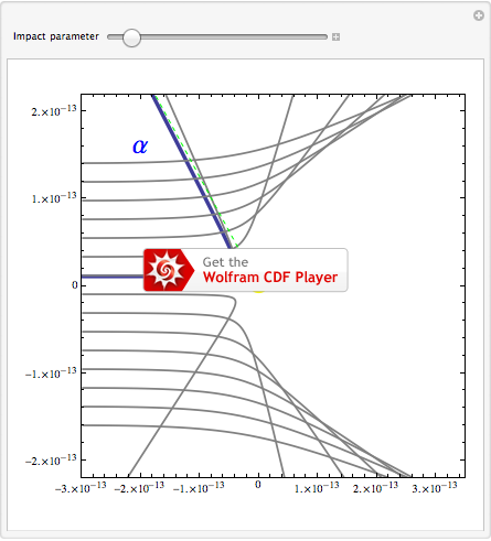
Experiments in Ernest Rutherford’s laboratory, carried out by Hans Geiger and Ernest Marsden in 1909, directed a beam of 6 MeV alpha particles, produced by radioactive disintegration, at a very thin gold foil, just the thickness of several atoms. The surprising result was that a small fraction of the alpha particles was scattered at large angles. Rutherford estimated that the scattering centers were very small, something less than 10-14 cm in diameter. It is now known that nuclear radii are typically of the order of several times 10-13 cm. The unit 10-13 cm is known as 1 fermi (fm), which can also be interpreted as 1 femtometer. The following CDF is an idealized representation of the scattering of alpha particles from a gold nucleus, based on the Demonstration “Rutherford Scattering” by Enrique Zeleny:
In 1911, Rutherford proposed the “nuclear model of the atom”. As we now understand it, a neutral atom of atomic number Z consists of a compact, nearly point-like, positively charged nucleus +Z e surrounded by a cloud of Z negatively charged electrons, each with charge –e.
This is where Niels Bohr now enters the picture.

Niels Henrik David Bohr (1885–1962) was born in Copenhagen, Denmark. His parents were Christian Bohr, a professor of physiology at the University of Copenhagen, and Ellen Adler Bohr, who came from a wealthy Danish Jewish family prominent in banking and parliamentary politics. His brother Harald Bohr became a prominent mathematician, noted for his work on Dirichlet series and the distribution of zeros in the zeta function. He introduced the concept of almost periodic functions. Both Harald and Niels were enthusiastic football (meaning soccer) players. Harald played for the Danish national team in the 1908 Olympics. Niels’ son, Aage Bohr, also became a physicist, who shared the 1975 Nobel Prize for his discoveries on nuclear structure. Bohr founded the Institute for Theoretical Physics at the University of Copenhagen, which was visited by all the major figures in the development of quantum mechanics. The Niels Bohr Institute, as it is now known, is still going strong.
Bohr spent a year as a postdoctoral student in Rutherford’s laboratory in Manchester. No doubt influenced by Rutherford’s nuclear model, he adapted the quantum concepts introduced by Planck and Einstein to propose a model of the atom as a miniature Solar System with electrons orbiting the nucleus. Three classic papers, published in Philosophical Magazine, summarize Bohr’s atomic theory:
[1] N. Bohr, “On the Constitution of Atoms and Molecules, Part I,” Philosophical Magazine, 26, 1913 pp. 1–25.
[2] N. Bohr, “On the Constitution of Atoms and Molecules, Part II: Systems Containing Only a Single Nucleus,” Philosophical Magazine, 26, 1913 pp. 476–502.
[3] N. Bohr, “On the Constitution of Atoms and Molecules, Part III: Systems Containing Several Nuclei,” Philosophical Magazine, 26, 1913 pp. 857–875.
We will next present the content of Bohr’s atomic theory. His original arguments have been modified to take advantage of a century of pedagogical experience and also some applications of Mathematica.
Bohr proposed that spectral lines arise from transitions between discrete energy levels of atoms. Building on the ideas of Max Planck on black body radiation and Albert Einstein on the photoelectric effect, a transition between two atomic energy levels E1 and E2 is associated with the absorption or emission of a photon of frequency ν (wavelength λ=c/ν, where c=2.9979 x 1010 cm/sec, the speed of light) according to the relation
![]()
where h is Planck’s constant, 6.626 x 10⁻²⁷erg sec. (We will use cgs and Gaussian electromagnetic units in this article for historical continuity.) For E2 > E1, this represents the emission of a photon as the energy of the atom decreases from E2 to E1 or the absorption of a photon of the same frequency as the energy increases from E1 to E2. This is also in accord with the Rydberg–Ritz combination principle (1906), which states that the spectral lines of any element will exhibit frequencies that are either the sum or the difference of the frequencies of two other lines. Applied to the Rydberg formula for hydrogen, it now follows that the discrete—we can now call them quantized—energy levels of a hydrogen atom have the form
![]()
which are negative values since they correspond to bound states of the atom. The integers labeling the energy states (n = 1, 2, 3, …) are called quantum numbers.
Bohr turned next to the specific case of the hydrogen atom, consisting of a single electron in interaction with a single proton whose mass is approximately 1836 times greater. The attractive Coulomb force between the two particles, varying as the inverse square of their separation, is exactly analogous to the gravitational attraction between a planet and the Sun. Bohr exploited this analogy with the Kepler problem to picture the hydrogen atom as a miniature version of the Solar System. In bound states, the electron should orbit the proton in an elliptical trajectory, with the proton at one focus. Bohr considered the simplest case of a circular orbit with the coordinate origin fixed at the position of the proton.
According to the virial theorem for an inverse-square force law, such as the Kepler problem and its electrical analog, the proton-electron system, we have T = -½V, where T is the kinetic energy and V the potential energy. The kinetic energy can be expressed in a form applicable to a circular rotating system, as ![]() , where L is the angular momentum of the electron, m its mass, and r the radius of the orbit. The potential energy is, by Coulomb’s law in Gaussian units,
, where L is the angular momentum of the electron, m its mass, and r the radius of the orbit. The potential energy is, by Coulomb’s law in Gaussian units,![]() , where ±e are the charges of the proton and electron, respectively. By the virial theorem, the total energy E = T+V can be expressed either as E = ½ V or E = –T. In terms of the Rydberg energy formula, we can then write
, where ±e are the charges of the proton and electron, respectively. By the virial theorem, the total energy E = T+V can be expressed either as E = ½ V or E = –T. In terms of the Rydberg energy formula, we can then write
![]()
To obtain a solution, we need a third relation. This can be provided by Bohr’s correspondence principle, which states that in the limit of large values of the quantum numbers, a quantum system will approach classical behavior. In this application, Bohr reasoned that, for large values of n, the frequency associated with a transition n –> n+1 will approach the classical frequency of the radiation emitted by an electron in a circular orbit. It is convenient to refer to the radian frequency
![]() From mechanics,
From mechanics, ![]() Noting that
Noting that ![]() for large values of n, we can substitute in the Rydberg formula to obtain
for large values of n, we can substitute in the Rydberg formula to obtain![]()
Now we can use Mathematica‘s equation solver to determine R, L, and r in terms of fundamental constants and quantum numbers:

The predicted value of the Rydberg constant is R = 109737cm-1. The slight discrepancy with the experimental value for hydrogen can be corrected by replacing m=me with the
reduced mass of the electron in hydrogen: ![]() . This gives, to high precision,
. This gives, to high precision,
RH = 109677.5810 cm-1. The value found above pertains to infinite nuclear mass. Using the best current values of the fundamental physical constants,
![]()
The result determining L actually introduces the profound concept of angular-momentum quantization. Dirac later wrote the constant h/2 π, which occurs frequently in quantum-theory formulas, as a single symbol ħ, pronounced “h-bar”. The quantum condition for the component of orbital angular momentum in any direction can then be written L = n ħ.
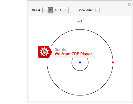
The third output of the Solve command above gives the radius of the electron’s orbit around the proton. For n = 1, we have the radius of the lowest energy state—the ground state—which is known as the Bohr radius and designated a0.
![]()
This was actually the first theoretical determination of the approximate magnitude of atomic dimensions. More generally, the electron orbital radius is given by rn = n2 a0, for n = 1, 2, 3, …. Following is a diagram showing the first few orbits. The proton is represented by a blue point, the electron by a red point. The radius of the innermost circle equals a0.

In contrast to a classical system, which possesses a continuum of allowed energy levels, a bound quantum system can exist only in one of a discrete (or quantized) set of energy levels. In a transition between the levels n and n‘, the electron somehow makes a quantum jump, accompanied by the absorption or emission of a photon of frequency ν = (En – En’) / h. The precise nature and mechanism of the “quantum jump” has been a controversial subject of philosophical speculation for an entire century.

Mathematica diagram showing a quantum jump.
The speed of the electron in the first Bohr orbit can be calculated from the angular momentum L = m v r. With L = ħ and r = a0 = ħ2 / m e2, we find v = α c, where α = e2 / ħ c ≈ 1/137, the fine-structure constant. This is comfortably within the non-relativistic domain (until we consider nuclei with large atomic number). Still, v is in excess of 2000 km/sec, which is a subtle hint that life on an atomic scale might be much different from what it is in the macroscopic world.
Hartree introduced a system of atomic units in 1928, in which ħ = m = e ≅ 1. This has the advantage of making atomic parameter values of the order of 1, rather than 10 to some large negative power. The unit of length, accordingly, equals a0, called 1 bohr. The unit of energy, called 1 hartree, can be constructed from e2/a0, equivalent to 27.212 eV. The energy levels of the hydrogen atom are then given by En = ![]() hartrees. The ground-state energy, when n = 1, equals -13.5984 eV. Thus the ionization potential of atomic hydrogen is 13.5984 volts.
hartrees. The ground-state energy, when n = 1, equals -13.5984 eV. Thus the ionization potential of atomic hydrogen is 13.5984 volts.
The Bohr model applies more generally to one-electron ions, with a nucleus of atomic number Z: Z = 1 for H, Z = 2 for He+, Z = 3 for Li2+, and so on. The potential energy is now generalized to ![]() , which leads to an energy of
, which leads to an energy of ![]() hartrees and an atomic radius of
hartrees and an atomic radius of ![]()
The Bohr atom represents a fundamental departure from the well-established classical theories of mechanics and electrodynamics. Most spectacularly, an electron in a Bohr orbit ought to radiate away its energy in about 10-11 seconds and experience a death spiral into the nucleus. I like to call this the “atomic Hindenburg disaster”. (The Hindenburg, a hydrogen-filled dirigible, crashed and burned in a famous disaster in 1937.) Nonetheless, the extraordinary agreement with the spectrum of atomic hydrogen must somehow justify this radical departure from classical physics.
Sommmerfeld and Wilson in 1916 generalized Bohr’s formula for the allowed orbits to a set of quantum conditions on action integrals, of the form
![]()
The Sommerfeld–Wilson quantum conditions reduce to Bohr’s results in the case of circular orbits, but now elliptical Kepler orbits are allowed as well, with the nucleus at one focus. In elliptical orbits, the momentum p can vary as a function of position.
For the hydrogen atom treated as a three-dimensional problem in spherical polar coordinates, there is actually a set of three quantum conditions:
![]()
where n, ℓ, m are integers with the ranges n = 1, 2, 3, …, ℓ = 0, 1, …, n – 1, m = –ℓ, –ℓ + 1, …, +ℓ (2ℓ + 1 values). The energy En is determined by n, which is called the principal quantum number. The value of ℓ, known as the azimuthal quantum number, determines the orbital angular momentum, but the precise connection must await the modern quantum-mechanical theory. The different values of m, called the magnetic quantum number, exhibit the phenomenon of space quantization, in which an elliptical orbit can be oriented in 2ℓ + 1 possible directions in three-dimensional space. (Full details on these results can be found in Appendix XIV of M. Born, Atomic Physics, 5th ed., New York: Hafner, 1935. The quantum number κ corresponds to what we designate as ℓ +1).
The n = 1 ground state is still a circular orbit, but the n = 2 level allows an elliptical orbit in addition to the circular one, with possible values ℓ = 0, 1. The n = 3 level has three allowed orbits, with ℓ = 0, 1, 2, and so on. The semi-major axis of the ellipse has the same value as the Bohr orbit, a = n2 a0. The semi-minor axis is then given by b = n(ℓ + 1)a0. The orbits for n = 1, 2, 3 are shown in the following Mathematica Demonstration:

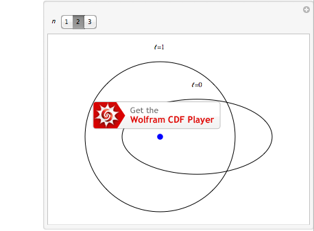
For a given n, the multiplicity of values of ℓ and m imply that there are, in total, n2 allowed orbits. The energy level En is said to be n-fold degenerate.
The atomic theory of Bohr, generalized by Sommerfeld and Wilson, is known today as the Old Quantum Theory, to distinguish it from modern quantum mechanics, which dates from 1925.
Circulating electric charges give rise to magnetic moments, in this case obeying the laws of classical electrodynamics. The general relation is μ = ![]() L. Thus an orbiting electron with one unit of angular momentum has a magnetic moment equal to μB = e ħ/2m c ≈ 9.274 x 10⁻²¹ ergs/gauss, which is known as a Bohr magneton.
L. Thus an orbiting electron with one unit of angular momentum has a magnetic moment equal to μB = e ħ/2m c ≈ 9.274 x 10⁻²¹ ergs/gauss, which is known as a Bohr magneton.
Many atomic spectral lines appear, under sufficiently high resolution, to be closely spaced doublets, a prime example being the yellow sodium D-lines, a doublet at 588.995 and 589.592 nm. Uhlenbeck and Goudsmit proposed in 1925 that this was due to an intrinsic angular momentum possessed by the electron (in addition to its orbital angular momentum) which could have just two possible orientations. This property, known as spin, occurs as well in other elementary particles. Spin and orbital angular momenta are roughly analogous to the daily and annual motions, respectively, of the Earth around the Sun. To distinguish spin from orbital angular momentum, we designate the corresponding quantum numbers as s and ms, instead of ℓ and m, which we now modify to mℓ. For electrons, s always has the value ½, meaning that its intrinsic angular momentum equals ½ħ. Correspondingly, ms has two possible values, ±½. The electron is said to be a “spin-½ particle”. Particles with spin equal to an odd half-integer are known as fermions. By contrast, particles with integer values of spin, such as the photon with spin 1, are called bosons.
A charged particle with spin also exhibits a magnetic moment, given by the slightly generalized relation
![]()
where S here means the intrinsic angular momentum, equal to ½ħ for the electron. It turns out that the g-factor for electron spin is equal to 2, so that the spin magnetic moment is also equal to 1 Bohr magneton, μB. Interactions between the orbital and spin angular momenta give rise to fine structure splittings of spectral lines, which are smaller in magnitude than the energies of orbiting electrons by a factor of the order of α ≈ 1/137, the fine structure constant.
Wolfgang Pauli proposed his exclusion principle in 1925. For fermions in a quantum system, such as the electrons in an atom or molecule, all the individual quantum states can be, at most, individually occupied. No such restriction applies to bosons; any number can occupy each quantum state. An example is a Bose–Einstein condensate, in which almost all the particles in a system occupy the ground state.
When applied to the electrons in an atom, the exclusion principle requires that every electron be described by a unique set of quantum numbers: n, ℓ, mℓ, ms. No two electrons can have the same set. The values of ℓ are usually designated by a code (originating in the classification of spectral lines, but no longer so limited): ℓ = 0 is designated s (not to be confused with the spin angular momentum), ℓ = 1 is designated p, ℓ = 2 is d, ℓ = 3 is f (this continues for higher angular momenta, but we will not need them here).
A complex atom can thereby be represented as a central nucleus surrounded by its electrons moving in Bohr–Sommerfeld orbits. The logos of the International Atomic Energy Agency and the former U. S. Atomic Energy Commission are both idealized versions of such pictures:

The structure of the periodic system of the elements could be rationally explained for the first time on the basis of the Old Quantum Theory. In accordance with the Aufbau principle, as the atomic number is increased, electrons successively occupy the lowest available Bohr–Sommerfeld orbits, taking account of the Pauli exclusion principle, which restricts each set of quantum numbers n, ℓ, mℓ, ms to, at most, a single electron. This produces the familiar shell structure of atoms. Complete shells, containing all values of the quantum numbers up to certain combinations of n and ℓ are occupied, appear to confer an enhanced stability to a set of atoms with the “magic numbers” Z = 2, 10, 18, 36, 54, 86, and 118. These are the so-called noble gases: helium, neon, argon, krypton, xenon, radon, and the synthetic transuranium element 118, discovered in 2006.
The following “staircase form” of the periodic table was proposed by Bohr in 1921:

Bohr supported Mendeleev’s original prediction that there was a missing element with Z = 72, chemically similar to zirconium. It was first isolated in 1923 as an impurity in zircon by Danish chemists in Copenhagen. This led to the element being named hafnium (Hf), which was the Latin name for Copenhagen. The element with Z = 107 was synthesized in 1981, and named bohrium (Bh) in honor of Niels Bohr.
The picture of the atom based on the Sommerfeld–Wilson quantum conditions and Bohr–Sommerfeld orbits of electrons is now known as the Old Quantum Theory. Despite its number of successful applications, the theory suffers from some serious flaws. To cite one, angular momenta are usually too large by one unit of ħ. For example, the hydrogen atom ground state is known to be zero rather than ħ. Zero angular momentum might be accomplished with a “pendulum orbit”, in which the electron oscillates linearly through the nucleus. This was, however, usually ruled out in the Old Quantum Theory because it involves collisions of the electron with the nucleus. Also, the theory is inconsistent with known behavior of atoms as nearly spherical particles. Although the Bohr model might have been able to sidestep the “Hindenburg disaster”, it can not avoid what might be called the “Heisenberg disaster”. By this we mean that the presumption of well-defined orbits is completely contrary to modern quantum theory, in particular the Heisenberg uncertainty principle, which states that the position and momentum of a particle cannot simultaneously be known exactly.
In addition, the Bohr theory was unable to produce any quantitatively valid results for atoms and ions containing more than one electron, most notably the helium atom. And it was a complete disaster in attempted applications to molecules. We should, however, mention the heroic effort of J. H. Van Vleck in his doctoral thesis (1922) to construct a model for helium, in which two Bohr orbits move in planes crossing at an angle of 88°. This gave a calculated ionization energy in approximate agreement with the experiment.
Despite its failings, the Old Quantum Theory was an important transitional step in the development of the modern picture of the atom. The reigning theory is now quantum mechanics, which emerged, beginning in 1925–1926, with major initial contributors being Werner Heisenberg, Erwin Schrödinger, and P. A. M. Dirac.
This pretty much concludes our account of Niels Bohr’s contributions to atomic structure. To his everlasting credit, he enthusiastically embraced the new quantum mechanics and his Theoretical Physics Institute became a shrine for the “Copenhagen interpretation of quantum mechanics”.
Bohr, largely in collaboration with Heisenberg, developed a viewpoint whose principal tenet was the hypothesis that quantum mechanics can usually predict only probabilities of atomic events. Variables thus do not have definite values until they are actually measured. In mathematical terms, a measurement results in “collapse of the wave function”. Einstein, for one, could never accept this rejection of objective reality (“Do you think the Moon isn’t there when you’re not looking?”). This led to an extended series of arguments between Bohr and Einstein, which actually produced many fruitful insights into some finer points of quantum theory and relativity. The controversy on the metaphysical foundations of the quantum theory continues even to this day, with concepts such as entanglement and decoherence becoming notable topics for consideration. Related to these is the possibility of quantum computation, in which two-valued bits are replaced by complex continuously variable qubits. Still, most practicing physicists go about their quantum-mechanical computations, blissfully unconcerned about the underlying metaphysics, as recommended by the advice, “Just shut up and calculate!”
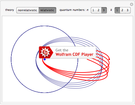
The subsequent theoretical treatment of the hydrogen atom by successively advanced versions of quantum theory is well covered in the existing literature. (See my Demonstration “Relativistic Energy Levels for Hydrogen Atom” embedded below.)
The most important modification was that the solutions of the Schrödinger equation for the hydrogen atom replaced the Bohr–Sommerfeld orbits by atomic orbitals, three-dimensional probability amplitudes for the distributions of electrons in space. (Explore the following pair of Demonstrations: “Visualizing Atomic Orbitals” and “Hydrogen Orbitals“, by Guenther Gsaller and Michael Trott, respectively.)
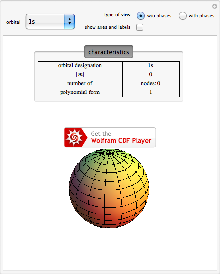
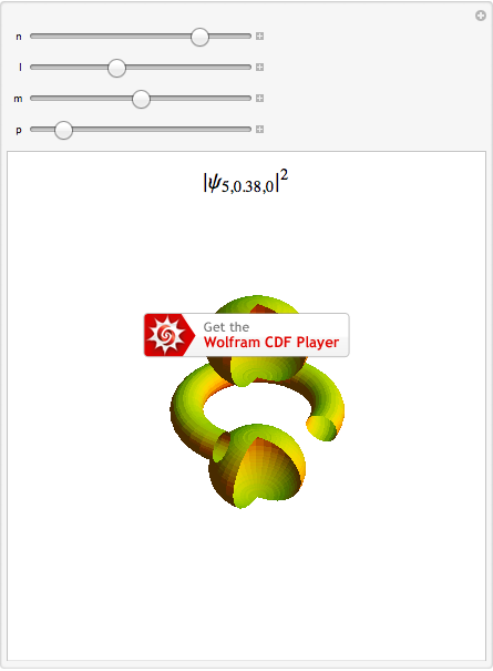
The energy levels of hydrogen-like systems are given by En = –Z2/2n2 hartrees, agreeing exactly with the Bohr model, but now the degeneracies of these energy levels are correctly accounted for. The solutions, depending on the three quantum numbers n, ℓ, m, are usually designated 1s, 2s, 2 p0, 2 p±1, and so on. Electron spin must still be put in “by hand”. Even though only the one-electron problem can still be solved exactly, the Schrödinger equation can be written down for any complex atom or molecule, and approximation techniques such as the variational method and perturbation theory could be applied to obtain highly accurate solutions. The concept of atomic and molecular orbitals is central to modern theoretical chemistry.
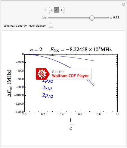
Dirac’s relativistic quantum theory of the electron automatically accounts for electron spin, with its g-factor of 2, spin-orbit coupling, the fine-structure of atomic energy levels (some of the degeneracies predicted by both Bohr and Schrödinger theories being thereby partially resolved), and, most dramatically, the existence of antimatter. Solving the Dirac equation gives the energies of a hydrogen-like system:

The energy now depends, in addition to the principal quantum number n, on the total angular momentum j = ℓ ± ½, the vector sum of orbital and spin contributions. (Remarkably, the same formula was obtained by Sommerfeld, in a relativistic generalization of the Old Quantum Theory, with κ instead of j + ½; explore my Demonstration “The Fine-Structure Constant from the Old Quantum Theory” embedded below this paragraph). The ground state is now designated 1 s½. The degeneracy in the n = 2 states is now partially broken, with 2 p3/2 higher in energy than 2 p½ and 2 s½. This constitutes fine-structure splitting, largely due to spin-orbit coupling. The 2 p½ and 2 s½ levels remain degenerate in Dirac theory but, as we will see, they are ultimately split by the Lamb shift of quantum electrodynamics.
It is interesting to expand the above energy formula in powers of the fine-structure constant α:

The first term gives the relativistic rest energy of the electron, m c2. The second term simplifies, in atomic units, with m = 1 and c2 α2 = 1, to –Z2/2 n2, reproducing the Bohr–Schrödinger formula. The complicated third term then accounts for relativistic corrections that cause the fine-structure splittings. It can be written more compactly as
![]()
Next came quantum electrodynamics (QED), which was also first pioneered by Dirac. It was later turned into the most spectacularly accurate physical theory in existence, with computational methods developed by Schwinger, Feynman, Tomonaga, and Dyson in the 1950s. In 1947, Lamb and Retherford measured the energy difference between the 2 s½ and 2 p½ states predicted to be degenerate by the Dirac theory. The Lamb shift, of the order of 1057 MHz, is due to the interaction of the electron with the vacuum state of the radiation field. QED is able to reproduce its magnitude to better than one part in 108. Also QED was able to account for the “anomaly” in the electron-spin g-factor. Its observed value is actually g ≈ 2.00232. Schwinger derived the first-order correction, giving
![]()
A more complete computation gives a value agreeing with the experiment to 1 part in 1012.
Finally, we describe the hyperfine structure of the hydrogen atom. The proton, like the electron, has an intrinsic angular momentum of ½ħ but a magnetic moment about 1000 times smaller than the electron’s. In the ground electronic state, a transition between the antiparallel and parallel electron-nuclear spin orientations produces a photon of 1420 MHz radiation, which falls in the microwave region, equivalent to a wavelength of 21 cm. The transition will occur in an isolated hydrogen atom approximately once every 107 years. Still, there are enough hydrogen atoms in a galaxy, including the Milky Way, for this transition to be detectable on Earth. It was first observed by Ewan and Purcell in 1951. In radio astronomy, radiation from hydrogen atoms is an important tool in the study of structure and dynamics of distant galaxies.
In the words of Arthur Schawlow, “The spectrum of the hydrogen atom has proved to be the Rosetta stone of modern physics: once this pattern of lines had been deciphered much else could also be understood.” We have followed this process, beginning with the primitive four-line visible spectrum of hydrogen, and culminating in measurements sensitive enough to detect the Lamb shift.
Download this post as a Computable Document Format (CDF) file.


Bravo!
Very, very fine modeled a history of science theory evolution. Thanks and regards.
This Comment is a reply to several questions and suggestions on my Blog commemorating the 100th anniversary of Neils Bohr’s atomic theory.
Michael Frayn’s award-winning play Copenhagen, produced in 1998, was an attempt to reconstruct what actually took place during Werner Heisenberg’s visit to Neils Bohr in 1941, during the Nazi occupation of Denmark in World War II. Heisenberg had worked at Bohr’s Institute for Theoretical Physics for several years beginning in 1924 and, by all accounts, they had a very warm personal friendship. Heisenberg, in collaboration with Bohr, were the principal creators of the Copenhagen Interpretation of quantum mechanics. Bohr’s half-Jewish ancestry placed him in a rather delicate position in the wartime political environment. There is no general agreement on what was actually discussed between Heisenberg and Bohr (another manifestation of the Heisenberg uncertainty principle?). Heisenberg, the head of the German atomic bomb project, hinted on the technical difficulties of the project. He may have judged the possibility of a uranium fission weapon as unattainable or that it might succeed if the war lasted long enough. He tried to engage Bohr on the morality of physicists devoting themselves during wartime to weapons such as the atomic bomb. Some speculation was that the purpose of Heisenberg’s visit was intelligence gathering: an attempt to determine if Bohr had any knowledge of the Allies’ progress on uranium fission.
Bohr and his family escaped from Denmark in 1943, narrowly avoiding arrest by the Nazi occupation forces. He worked for a time on the Manhattan Project at Los Alamos, under the alias “Nicholas Baker.” After the War, Bohr was a vigorous proponent for international cooperation on nuclear energy. He was influential in the creation of the International Atomic Energy Agency and received the first Atoms for Peace Award in 1957.
Bohr, in collaboration with John Wheeler, derived a simple relation predicting which nuclei were likely to undergo spontaneous fission: Z^2/A >2(a_S/a_C), where a_S and a_C are the surface and Coulomb energy factors, respectively. With a_S ≈18 MeV and a_C ≈ .472 MeV, Z^2/A equals about 50. See:
N. Bohr and J. A. Wheeler, “The Mechanism of Nuclear Fission,” Phys. Rev. 56, 426-450 (1939).
Another subject of comments I received concerned the relation between Bohr orbits and de Broglie matter waves. It turns out that the allowed orbits contain exactly an integer number of de Broglie wavelengths. Refer to the two Demonstrations: http://demonstrations.wolfram.com/BohrsOrbits/ and http://demonstrations.wolfram.com/ElectronWavesInBohrAtom/
On Bohr’s first postulate
In the last fifty years, educationists have observed a few common misunderstandings among students, young and grown-up. They seem to be global and cause adverse effect on the liking for physics in students. So I am working on conceptual aspects of Newtonian mechanics for nearly 35 years and also focus on related topics like the planetary motion and Bohr’s theory of Hydrogen atom. So I would like to draw attention of readers to his first postulate and reconsider it in view of my following statement.
As per the first postulate – the centripetal force for the motion of electron, around the nucleus of Hydrogen, is provided the electrostatic force of attraction between the electron and the positively charged nucleus. For 100 years, we have been using it without any real difficulty. But I noticed a conceptual difficulty, describing it first in a quarterly of UNESCO in Jan-Mar 1980. Let me raise it again here.
We use the electrostatic force in the concept of electrical potential energy also, where the motion of charged particle is *along the line of action of force*. Thus we use one and the same force for two different modes of motion – i) motion along the line of action in the potential energy and ii) motion perpendicular to the line of action in Bohr’s theory. Frequently the question that comes to mind is: If one and the same force is used in two totally different modes of motion, WHY there are no conditions to allow only required mode to take place and not the other mode? I think that this question requires serious attention of educationists as well as physicists. Feel free to discuss more on this point.
I read your beautiful post on the history of the hydrogen atom; I like it, and it is a pity that you gave up (if I understand correctly) the idea of writing a larger treatise. About the two main components of physics, i.e. experiments and mathematics, I am more inclined to the second. I have studied most of what you write in the post many years ago. After, I have never used and I have never taught Bohr-Sommerfeld theory, but only Quantum Mechanics. But it was nice to see again in your post ( I have forgotten) that Nature started to reveal his secrets with the four lines in the visible region of the hydrogen spectrum; of course it is amazing and gives us an almost religious feeling that in galaxies, far from us ten billions of light years, infinitesimal spin-flips of electrons of H atoms, produce photons that reach us, and inform us about their origin. I am sure that you agree with this feeling.
Great post.
If you like this, you may like my 4D version of an alternative form of the periodic table- now available as a Wolfram Cloud application (if you have and are logged in on a WolframID
or here as a CDF if you have Mathematica or the free CDF player:
Greg
Prof Prem raj Pushpakaran writes — 2019 marks the 100th year of the discovery of positively charged stable subatomic particle, Proton!!!