Mathematica 9 has just been released with many new or enhanced capabilities for image processing. You can perform morphological operations, color manipulation, segmentation analysis, feature detection, and more, most of which can be applied to the new Image3D object as well.

A byproduct of this whole ecosystem is that now it is easier than ever to use Mathematica to create and apply effects to your images.

Two Mathematica super functions that can be used to apply transformations directly to an image are ImageApply, which is a pixel operator, and ImageFilter, which considers the pixel as well as a neighborhood of pixels around it and works as a local filter.

For example, you can remove the blue channel and perform a gamma correction only on the green channel by doing the following:

Or, design a custom filter to average the values in the blue channel only over a specified neighborhood range:

Some common functions are already included with an internally optimized version; such is the case for the mean filter, which is named, not unexpectedly, MeanFilter.

Using this in combination with the duo ColorSeparate/ColorCombine, we can write a much more readable and efficient version of the filter above.

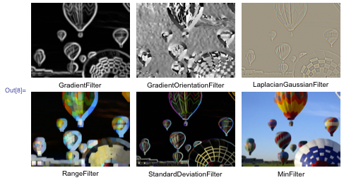
Here is a subset of the other filters present in Mathematica 9.

And here are Mathematica 9’s embedded image effects.

Mathematica‘s image processing functionality allows you to apply masks, for example, to create vignette effects. First we need to generate the mask. I am going for a simple shading at the corners, obtainable using a Gaussian mask.

Now we only need to adjust the mask dimensions to the ones of our original image so that it is possible to combine them.

We can even change the mask’s color.

This procedure is very straightforward, but a bit rough. What if we want to perform some fine tuning of our color mixing?

The general idea would be to implement an expression like: (1 – α) mask + α color.

Or, if we want to maintain the pure black at the corners, simply: mask + α color.

We can do the above using image arithmetic functions such as ImageSubtract and ImageMultiply that are now updated to work with a list of channel values.

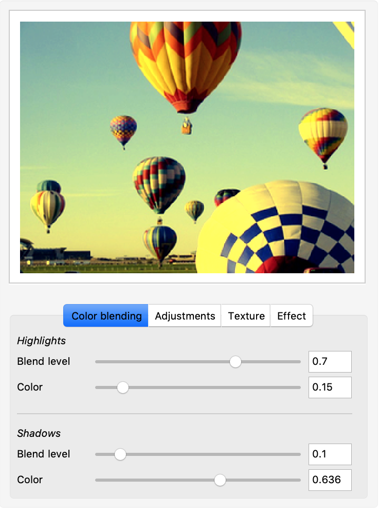
With a little more effort, it is possible to put many more effects together in a single, interactive panel.

Using the luminosity as parameter, I implemented a blending effect limited to the dark or light areas. With ImageAdjust we can fix contrast, brightness, and gamma, and ImageMultiply can easily handle applying textures.

As a final effort, I would like to create something totally different from what we have just seen: a filter that transforms my picture into something similar to a comic, with only black and white and a uniform filling pattern for the gray area.

I don’t want too much black in the image, so I try to convert our image into black and white with a low threshold. Then we need the part in the middle, the gray area; this we can get with Binarize too.

To generate the repetitive pattern that we will use to fill the gray area, we use the Mod function.

As a final step, we use an AlphaChannel to make gray pixels fully transparent so that the pattern can be seen through the mask.

The beautiful thing in Mathematica is to be able to play interactively with your code. Here is a CDF where you can see the effect of a parameter change in real time. I also added a control to change the background pattern and an option to emphasize the edges in the image.

We have just seen how to create several basic image effects with Mathematica. Using these as building blocks, it is possible to reproduce the filters embedded in popular applications on the market like Instagram or Hipstamatic with a little more effort. The big difference with Mathematica is that you know exactly what’s going on behind the curtains, and amazing results can be achieved with only few lines of simple code.

Download this post as a Computable Document Format (CDF) file.