Volumetric Rendering of Colliding Galaxies
The physics involved in simulating galaxy collisions can be extremely complex. The most accurate simulations take into account not just points representing stars, but also magnetic fields and invisible dark matter, as well as n-body interactions allowing the individual stars to interact with each other. These complex simulations are usually carried out on large-scale supercomputers over long periods of time. One of the more interesting aspects of galaxy collisions is that they can create density variations resulting in all kinds of emergent structure. Density waves can develop that lead to star formation from compressed gas clouds.
A couple of years ago, I wrote a Demonstration that provides a simplified solution to galaxy collisions. This Demonstration is designed to run in real time inside a Manipulate, so the problem has been simplified by removing n-body interactions, dark matter, magnetic fields, and so on. Basically, it treats the two galaxies as large point masses with lots of massless test particles orbiting them. The test particles respond only to the two galaxy “centers.” In a real galaxy collision, the chances of two stars getting close enough to each other to interact directly is very remote, so it’s not too far of a stretch to ignore this effect for a first-order approximation. The more stars that are included in the simulation (by minimizing the star separation parameter), the more intricate the results (and the more computationally intense). In fact, as more stars are added, it becomes easier to see density variations where many test masses cluster together, but it still looks very discrete. Real galaxies, like the Milky Way, can have hundreds of billions of stars. Trying to carry out a point simulation with that many stars becomes a bit taxing on most home systems, and definitely exceeds the time constraints of a real-time dynamic tool like Manipulate. So how can we better visualize these density variations? I decided to try to modify my Demonstration to use one of the new features in Mathematica 9, namely volumetric rendering. This way, we can simulate the galaxy collisions with fewer numbers of points, but render the results as if there were billions of stars, resulting in a more realistic and informative visualization.
To see the difference, here is a frame from a simulation I ran using the original code:

And here is a frame from the same simulation, but using volume rendering:

Volumetric rendering is a tool used to visualize datasets that are 3D in nature, with variations in density displayed using varying opacity. Since the individual “stars” in the Demonstration are more representative than literal (i.e., each point represents a larger collection), it should be an easy thing to just bin these points and construct a 3D volumetric dataset composed of voxels, where the opacity is a function of the number of test masses in each voxel. The result should look more like a smooth cloud than a discrete set of points and achieve the desired goal much more effectively. It turns out that the changes to the code were quite minimal. I won’t go into detail describing all of the code in the Demonstration, since most of it involves the mechanics, but I will describe the important aspects. Originally, the Demonstration’s Draw function was essentially just a Graphics3D that drew a couple of multi-point clouds along with some styling information:

In the new version, I changed Draw to render densities using Image3D instead:

Now, due to the more complicated data being rendered and the large values of points needed, this code is not fast enough to use in real time via Manipulate, but Manipulate still provides a nice interface for tweaking the parameters and then running the simulation as an animation. By exporting the resulting frames, you can convert them to a video format of your choice.
The volume-rendered results are much more informative. With the use of a color function, the density variations become more obvious and immediately comprehensible.
Let’s illustrate this with an animation. Here is a version using point clouds:
Here is the version using volume rendering:
Using the volume rendering feature along with image processing in Version 9 can result in some stunning visualizations, right on your desktop.
Download this ZIP file which includes the blog post as a Computable Document Format (CDF) file and a notebook with sample code.

Very nice visualization, perhaps one day you find the time to describe the mechnics behind it some detail.
The mechanics are referenced from the original Demonstration in the Details section. The code has be translated to Mathematica, updated, and an interface added, but the same ideas still apply.
M. C. Schroeder and N. F. Comins, “Galactic Collisions on Your Computer,” Astronomy, 16(12), 1988 pp. 90–96.
Very intriguing. I can imagine all kinds of mixing of dynamic “fluids”! Like Brownian diffusion distributions. I intend to persue graphic additions to my papers in the near future to enhance receptance and creditability for my descriptions of analogies. GHB