I was browsing Mathematica user communities for original projects and came by the following question: “How can I calculate a jigsaw puzzle cut path?” Such creative problems are in abundance at our user forums, the Wolfram Demonstrations Project, and The Mathematica Journal, which tells me that Mathematica, at its heart, is a conduit for creativity: it’s a programing language that likes the challenge of convoluted problems and inspires elegant, often unexpected solutions.

In its essence, a jigsaw puzzle is a tiling or tessellation, which means there are no gaps or overlaps between the pieces. Moreover, every piece is unique and has a definite place in the puzzle. Uniqueness is achieved by making a piece be a part of a large image, have a specific shape, or a combination of these. There are many approaches to producing such patterns. For instance, this single mathematical formula from our graphics examples produces a beautiful tessellation:

However, since this question was asked on Mathematica Stack Exchange, a young, modern technical Q&A site, it was very specific in accordance with the community rules. Here are the author’s requirements:

• All pieces must be unique to preclude placing a piece in the wrong spot.
• Pieces must be interlocking such that each piece is held by adjacent pieces.
• It must be possible to generate different paths (sets) for a specific shape that are not merely rotations or reflections of the first.

Additionally, the author of the question notes that he seeks original designs alternative to typical mass-produced shapes.

The question grabbed my attention. At first I thought that if we want to recreate interlocking parts and non-standard shapes and guarantee a perfect tessellation, the task could be a bit elaborate. Yet as it often happens with Mathematica, a solution was right around the corner.

First we start with a tessellating tiling producing more or less unique shapes. A Voronoi diagram (or Dirichlet tessellation) is a good start because it can be constructed on a set of random points. This will guarantee uniqueness of shapes with high probability. We could use the Computational Geometry Package to build a VoronoiDiagram, but there are other perhaps less known ways worth sharing. For example, from an image processing angle this can be achieved with the DistanceTransform function. But perhaps the simplest way is using Mathematica‘s native graphics functions, such as ListDensityPlot.

Such graphics objects consist of graphics primitives and their options. Here Voronoi cells are represented by the Polygon function; this is a typical element:

Use InputForm[gr] to see the complete structure.

The next step is to replace the sides of these polygons with interlocking parts. These can be achieved with splines. In addition to two endpoints of a polygon side, we need to provide three more points: a midpoint to mark where the interlocking part is and two extra points to wrap the spline around. Varying point positions and spline parameters, we can design an interlocking part in a shape we like. Try this with the interactive CDF (Computable Document Format) below:

Dragging locators of endpoints in the app above will frequently flip the lock direction. This emphasizes that for every pair of points, the lock orientation will be chosen randomly. The lock size is proportional to the distance between the points. For short enough distances the spline line will disappear and leave the polygon side intact to make sure that the lock is not too small. That would make cutting it out with scissors difficult. Once we find the satisfactory geometric parameters, we use them to define the lock function:

Next we define a function that will extract from a Voronoi diagram all pairs of points representing the polygons’ sides:

Let’s see how these functions work. We will use MorphologicalComponents and a few other image processing functions to color the polygons, now with locks.

This alone could be a puzzle design if not for a few problematic issues. There are some overlaps, some pieces are too small, and sometimes locks appear on the sides with no adjacent pieces. To fix this we introduce an interactive interface where slight discrepancies can be manually fixed. This also provides an excellent tool for adjusting, removing, and adding polygons to achieve the best visual design. I added the ability to overlay the cutting paths over a few photographs I’ve taken over the years:

I enjoy Mathematica‘s ability’s to make images part of the code. You can replace them with your own photographs. Please note that the lock and extract functions and variable iml need to be evaluated first for the code below to work. You can always add them explicitly in the body of Manipulate or via its option Initialization.

You can drag polygons around with your mouse and add or remove them with Alt+Click. The interface is self-explanatory, so try various controls. When you like your design you can click the button “copy” to store your work in the clipboard. Then you can paste it into Mathematica or any other program that allows printing of images. To take full advantage of the application above, you need to have the free Wolfram CDF Player or Mathematica installed. Here is the preview of a single piece moved in a circular path through the puzzle. Note how other cells automatically adjust to it.

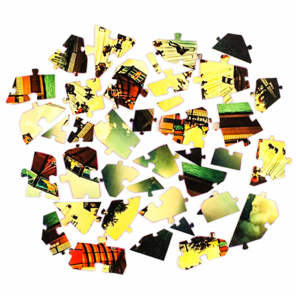
Now imagine helping your five-year-old solve a small and easy jigsaw puzzle that assembles into his or her favorite vacation moment or pet portrait. I was determined to go beyond pure computer design and into the real world. I used thick printing paper. Photo paper or even gluing an image to cardboard would be better for locking, but harder to cut. Manufactured puzzles are cut with a press, which produces several hundred tons of force, or a laser. I obviously resorted to scissors. It took me half an hour to cut all the pieces out, and I had a bit of trouble dealing with not-thick-enough paper, resulting in improper locking. But at the end it all was well worth the effort. Jigsaw puzzles are well-known for their great recreational value, and even served as escapism during the Great Depression, showing a remarkable number of sales. Here is my handiwork:

And next it is almost done. I used small adhesive tape on the printout back to fix every newly added piece. That helped to improve locking. And I did not look at the box!

Jigsaw puzzles have been around since the 1700s, with many old and modern masters cutting them from wood and showing unique styles in shaping the pieces. And though computers often cannot reproduce natural human art forms, the reverse is also true. A jigsaw master cannot reproduce by hand a Voronoi tessellation, which is quite a beautiful mathematical form.

But does this approach scale toward more intricate puzzles? Now imagine you are a puzzle designer or manufacturer with access to industrial cutting equipment. Then there’s no limit to what is possible with the help of mathematics, programming, and environment as well integrated as Mathematica. We can use Mathematica‘s native vector graphics objects or export them to other standard vector graphics formats. This allows for magnifying designs to arbitrary dimensions and printing large detailed puzzles similar to complex commercial editions that count thousands of pieces. The most challenging puzzles are monotone-colored, with the uniqueness of the pieces as a consequence of differently shaped locks. To add complexity, some puzzles are double-sided so it is not clear which is the top side of a piece. It would be very easy to design such puzzles with typical grid-like layouts, but we can go further. Mathematica covers all sorts of pure and applied scientific fields, and their methods can provide inspiration and tools for puzzle design. Let’s take graph theory as an example and built-in data for a famous fractal called the Sierpiński sieve or gasket.

With two lines of code we can replace the edges of a graph with our spline locks. I will modify our lock function to produce randomly shaped locks similar to commercial puzzles. Not only are the locks randomly tilted now, but their tips are also made randomly convex or concave by introducing an extra spline point. This will greatly reduce the probability of accidentally getting similar pieces.

Adjacent triangles of all sizes are counted as pieces here, so one strategy for assembling the puzzle is to start from larger central pieces. Locks can always be made more sophisticated by adding more spline points. I used graph functionality in this example purely for instructive purposes to show the easy mapping from network and spline objects. Here is equivalent functional programming code that produces a Sierpiński jigsaw puzzle of more than 3,000 pieces as a vector EPS image in a few seconds on an average laptop. Thanks to our growing library of over 8,000 Demonstrations, I could quickly find relevant code courtesy of Peter House.

And so we added to a puzzle the educational merit of naturally teaching the nesting construction of fractal structures. Often when I open a Mathematica notebook, I do not know where the adventure will take me—it is so easy to improvise and turn things into an experiment. Have fun designing, playing, and learning!

Download this post as a Computable Document Format (CDF) file.