In silico medicine, particularly through the use of finite element simulations, is revolutionizing patient-specific healthcare, especially in the musculoskeletal system. By creating detailed computational models of individual anatomy, finite element analysis enables precise simulation of biomechanical behavior under various conditions. This approach allows for personalized treatment strategies, offering predictive insights into how specific interventions—such as surgeries, prosthetics or rehabilitation plans—might affect the patient’s musculoskeletal health. Unlike traditional experiments such as in vivo or in vitro, in silico medicine refers to simulations where the experimental environment is recreated within the processor.

The term in silico comes from the main component of computers: the processor, which is made of silicon. With these simulation techniques, such as finite element simulations, it is possible to reduce the need for invasive procedures and physical testing by providing a noninvasive, cost-effective and highly detailed method to explore the complex interactions within structures like tendons, joints and bones. This innovation is paving the way for more effective, individualized treatments and a deeper understanding of biomechanical health.

Engage with the code in this post by downloading the Wolfram Notebook

In this example, we will explore a detailed demonstration of a finite element uniaxial test experiment applied to a tendon structure. The geometry, derived from medical imaging, highlights patient-specific outcomes. For simplicity, we will start with the anatomical database available in Wolfram Language:

The process begins with geometry analysis, accommodating both STL-like meshes and volumetric images commonly produced by clinical diagnostic imaging techniques. Following this, we will assign material properties to the tendon structure and simulate a load-bearing experimental scenario, focusing on its behavior during a uniaxial tensile test. This approach demonstrates the workflow for integrating patient-specific data into biomechanical simulations.

Calcaneal Tendon and Virtual Patient

The calcaneal tendon, or Achilles tendon, is the strongest and largest tendon in the human body, connecting the gastrocnemius and soleus muscles of the calf to the calcaneus (heel bone). It plays a vital role in enabling plantarflexion of the foot, a movement essential for walking, running and jumping. This tendon is capable of withstanding tensile loads of up to 12.5 times body weight during high-impact activities, such as running or jumping, and has an elastic modulus ranging from 1.2 to 2.0 GPa, allowing it to store and release energy efficiently. Typically, the tendon can tolerate strains of up to 8–10% before failure.

The Achilles tendon is prone to pathologies caused by overuse, acute trauma and age-related degeneration. Chronic overuse often leads to Achilles tendinopathy, characterized by pain, swelling and impaired function due to repetitive microtrauma. Sudden, forceful movements in sports can result in tendon ruptures, particularly in middle-aged individuals with diminished elasticity. Insertional tendinitis, inflammation near the tendon’s attachment to the heel, is another common issue, exacerbated by biomechanical stressors like Haglund’s deformity or improper footwear. Aging further reduces tendon elasticity, increasing susceptibility to microtears and ruptures, while overloading and biomechanical imbalances, such as overpronation, unevenly distribute stress, heightening the risk of injury.

In this context, in silico medicine plays a crucial role in clinical scenarios. By using computational models tailored to individual patients, clinicians can simulate the biomechanical behavior of the Achilles tendon under various conditions. This approach enables the prediction of injury risk, optimization of treatment strategies and design of personalized rehabilitation plans, all while reducing reliance on invasive procedures. The integration of in silico methods into clinical practice enhances our ability to address the complex challenges of Achilles tendon pathologies and improve patient outcomes.

The following example is structured into multiple sections. First, the “Imaging” section outlines the transformation of medical images into a virtual representation of the patient, utilizing several anatomical marker points. Next, the image is converted into a mesh, a structure suitable for finite element analysis (FEA). Finally, multiple FEAs are performed to examine the mechanical behavior trends and the impact of the pathology.

Imaging

The standard approach to patient-specific biomechanical assessment begins with medical imaging:

While handling the various medical image formats is beyond the scope of this text, all formats can be converted into grayscale volumetric images, where a specific threshold can be set to highlight the relevant tissue regions. To provide a broadly applicable example, we will start with the tendon morphology obtained from the AnatomyData of the anatomical structure entity in Wolfram Language:

This image showcases the volume rendering of the tendon, closely resembling the images produced by medical scans such as CT or MRI.

Next, we can convert this volumetric representation into a mesh suitable for FEA. The goal is to generate a mesh that is both sufficiently accurate and computationally efficient, balancing detail with a reasonable number of elements.

To achieve this, we can use the ImageMesh function with different methods. However, in all cases, the resulting mesh retains characteristics tied to the resolution of the original volumetric image. This is a common challenge when converting clinical images from medical equipment into digital models suitable for numerical computations:

A more effective approach involves analyzing the mesh structure in terms of its points. These points, now serving as markers on the tendon surface, can then be refined using smoothing algorithms, alternative meshing techniques or, given the tendon’s shape, a surface lofting approach to create a more structured representation.

Anatomical Markers

At this stage, it becomes clear that we can identify multiple contour lines at the same height, which can be utilized to construct a lofted surface:

The approach follows these key steps:

1. Define a fixed number of slices: Establish evenly spaced cross sections along the tendon’s height.
2. Extract points for each slice: For each cross section, collect all points at the corresponding height.
3. Generate contour lines: Create a line that interpolates through the extracted points for each slice.
4. Construct the loft: Connect the sequence of contour lines to form a smooth 3D lofted surface.

This method enables a structured and refined surface representation, improving the accuracy and smoothness of the final mesh while maintaining anatomical fidelity.

For convenience, let’s start with a rotation of the tendon to align it with a more intuitive coordinate system:

From Imaging to a Computational Mesh

Before creating the loft, we need to clean up the data. First, let’s ensure that each slice is precisely aligned along the loft’s direction (x coordinate):

As the second step, we need to ensure that each slice forms a closed loop, with points ordered sequentially to maintain a consistent structure:

Now, we aim to extract a reduced set of points to simplify the final mesh while maintaining an illustrative example. To achieve this, we will select a small number of marker points, ensuring a relatively simplified yet structured representation.

Additionally, we must ensure alignment of extracted points across all slices. To do this, we:

1. Start from the first slice and select points based on uniform angular distribution.
2. Translate the slice to the origin, which can facilitate alignment and ensure consistency.
3. Use a dynamic visualization element to interactively inspect and refine point selection.

This approach helps maintain geometric coherence while effectively reducing computational complexity:

This allows us to extract points that are aligned relative to the first slice:

Now, we have two sets of lines forming a grid that covers the tendon. This structured representation can be used to generate a mesh using OpenCascade, ensuring a well-defined and smooth surface reconstruction:

Let’s now ensure that each line forms a closed loop, maintaining continuity and consistency across the structure. This step is essential for generating a well-defined surface mesh:

We can proceed to generate the lofted surface using OpenCascadeShapeLoft:

Finally, we can mesh the lofted surface into a solid tetrahedral mesh, ensuring a volumetric representation suitable for FEA. This step converts the structured loft into a watertight 3D model, enabling accurate biomechanical simulations and structural assessments:

Finite Element Analysis

We aim to compute the stress and strain distribution within the material by simulating the mechanical stretching of a tendon. In this scenario, one end is fixed, while a load is applied to the opposite end. Physiologically, a tendon can experience forces exceeding 10 times the body weight.

The framework for structural FEA makes use of the SolidMechanicsPDEComponent, which is well described in the Solid Mechanics monograph. Let’s extract the coordinates of the two boundary sides, along with the load direction, which can be reasonably assumed to align with the tendon’s principal axis:

The typical loading scenario for the tendon involves a tensile load applied along its longitudinal direction, which can be represented by fixing an extremity and pulling the other one.

Tendons exhibit relatively high stiffness, which is often modeled using a Neo-Hookean hyperelastic model with a shear modulus with a typical range of 0.1–1 GPa:

The mechanical problem can be conveniently formulated using the SolidMechanicsPDEComponent function. Given the high nonlinearity of the problem and the large strains involved, we set up a parametric solver that depends on a load factor k (ranging from 0 to 1). This allows for a gradual increase in the applied load, ensuring better convergence while solving the problem:

To minimize the nonlinearities of the problem, a parametric solver can be configured to gradually increase the load. This approach is thoroughly explained in the Hyperelasticity monograph:

As shown in the following figure, the tendon is stretched along its principal direction, exhibiting a displacement with a stretch ratio of up to 200%:

This image illustrates the final deformed configuration resulting from the applied load. The gray-shaded geometry represents the undeformed tendon. Additionally, the deformed geometry is color-coded based on the equivalent strain, which is highest in the central region and gradually decreases toward the boundaries:

But what happens in the case of pathology? How does the mechanical response change when structural integrity is compromised?

Before investigating pathological conditions, we must account for the fact that tendons are highly transversely isotropic, with a significant load-bearing contribution from collagen fibers (which constitute up to 80% of the tendon structure) aligned along the loading direction.

Typically, this collagen fiber network exhibits a stiffness up to 20 times higher than the surrounding matrix, which is composed of elastin, cartilage, proteoglycans, inorganic components and other extracellular matrix elements. This strong anisotropic behavior plays a crucial role in the tendon’s mechanical response and load distribution:

Tendons are primarily composed of type I collagen fibers, which are highly organized and aligned along the loading direction. This fiber-reinforced structure enables tendons to efficiently transmit forces from muscles to bones while withstanding high mechanical loads—often exceeding 10 times body weight during intense physical activity.

The collagen matrix works in conjunction with proteoglycans, elastin and other extracellular components, contributing to the tendon’s viscoelastic behavior, allowing it to store and release energy efficiently. In pathological conditions, such as tendinopathy, collagen degradation and disorganization can lead to weakened mechanical properties, increasing the risk of injury or rupture:

Geometry Simplification

Before further investigating the influence of collagen fibers, let’s simplify the geometry to enhance computational efficiency. We can achieve this by extracting a 2D representation of the tendon by taking a cross-sectional slice from the 3D model:

The figure displays the 3D structure of the tendon along with a box highlighting its bottom half. This setup allows for a precise mid-section slice, enabling a clearer view of the internal structure:

Note that the intersection points are not evenly distributed, which may affect mesh quality. To ensure the best possible mesh, we need to remove points that are too close to each other, preventing overly small elements and improving numerical stability:

Before meshing, it is advisable to standardize the points. Specifically, by applying a threshold, we can filter out nearby points, ensuring a higher-quality mesh:

To better apply the pulling force, let’s consider a general uniaxial strain experiment, where the pulled side is clamped to a rigid support (i.e. a material with significantly higher stiffness compared to the tendon). This setup ensures a well-defined boundary condition, mimicking realistic loading conditions. Geometrically this can be identified as a triangle. So we can mesh the geometry:

As a result, we obtain a planar mesh with good quality. The mesh consists of two distinct domains: the tendon (red) and the pulling clamp (gray), each assigned different material properties.

Collagen Fibers’ Influence

Tendons can be viewed as fiber-reinforced materials, where the primary load-bearing components are the fibers, which exhibit significantly higher stiffness compared to the surrounding matrix:

This figure displays the deformed mesh, color-coded based on first principal stress. As observed, stress is particularly high in the central bottom region and gradually decreases towards the extremities. This distribution is influenced by both the thinning of the central region and the higher curvature in the bottom area, which, under the horizontal pulling load, experiences significant mechanical stress.

Pathology and Collagen Damage

From a mechanical perspective, tendon pathology is often characterized by a reduced ability of collagen fibers (the main load-bearing component) to transmit forces effectively. This degradation can lead to conditions such as tendinosis, tendinitis or even rupture, depending on the severity of the lesion, as detailed in studies from Arya and Kulig, 2010; Yin et al., 2021; and Freedman et al., 2014:

Mathematically, this can be represented as a localized alteration of the mechanical properties within a specific region of the tendon. This may include changes in stiffness, elasticity or failure thresholds, affecting the tendon’s overall ability to sustain loads:

As previously mentioned, fibers play a crucial role in the stiffness and load-bearing capacity of tendons due to their widespread distribution and significantly higher stiffness (up to 20 times greater than other components). Now, let’s investigate their influence on the tendon’s mechanical behavior using the simplified 2D mesh:

The plot illustrates the undeformed planar section of the tendon along with the fiber distribution, which is predominantly aligned along the longitudinal direction. The rainbow colors represent the damage properties, with the highest concentration (red) located in the central bottom region. This directly correlates with a reduction in mechanical properties, affecting the tendon’s structural integrity:

The relaxation of pathological fibers is clearly observed in the displacement field, with the pulled side exhibiting noticeable rotation. But how does this affect strain and stress distribution?

Both stress and strain play a critical role in injury risk and the progression of inflammation, making their evaluation essential for understanding the mechanical implications of tendon pathology:

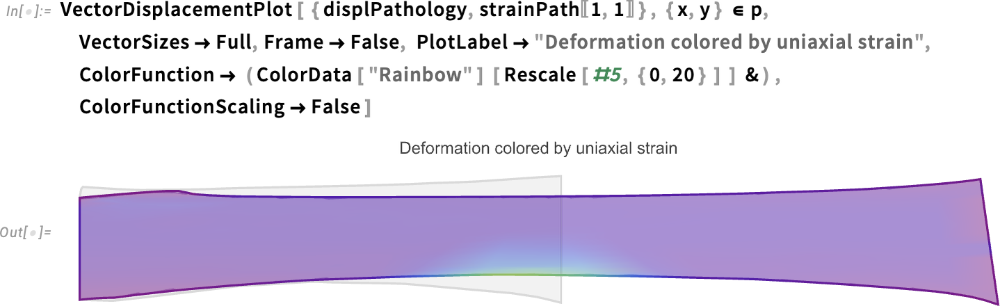
This figure illustrates how, due to the pathology, the stress is significantly higher in the bottom region. Additionally, the final deformation on the right side is more pronounced compared to the healthy case. Furthermore, it allows for a direct comparison of stress distribution between the healthy and pathological cases, highlighting the impact of the condition on the tendon’s mechanical behavior:

As we can see, stress slightly increases in the upper region, while it slightly decreases on the bottom side. Note also the increase near the damaged region. These effects warrant further investigation, particularly in relation to pathology progression.

Curious about the technical details? You can find all the relevant information on FEM and structural modeling on the PDEModels Overview reference page.

However, for a deeper analysis, you’ll have to stay tuned for the next post!