Two years ago we released Version 13.0 of Wolfram Language. Here are the updates in visualization and graphics since then, including the latest features in 14.0. The contents of this post are compiled from Stephen Wolfram’s Release Announcements for 13.1, 13.2, 13.3 and 14.0.

New Plot Types

New in Visualization (June 2022)

In every new version for the past 30 years we’ve steadily expanded our visualization capabilities, and Version 13.1 is no exception. One function we’ve added is TernaryListPlot—an analog of ListPlot that conveniently plots triples of values where what one’s trying to emphasize is their ratios. For example let’s plot data from our knowledgebase on the sources of electricity for different countries:

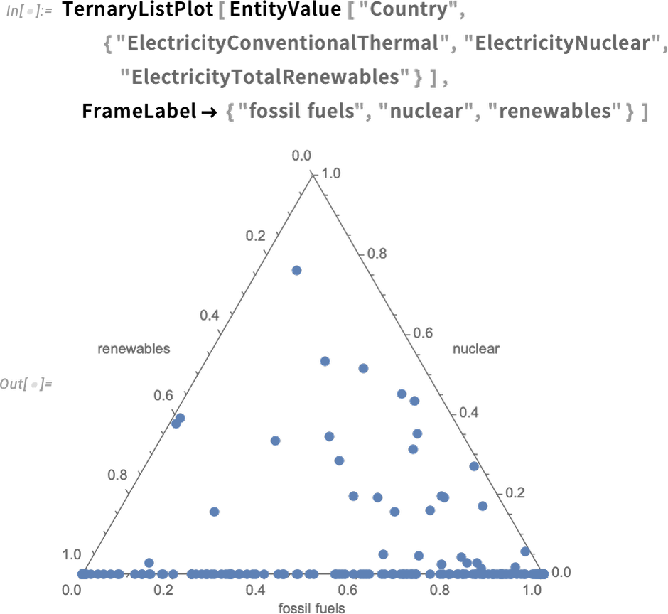
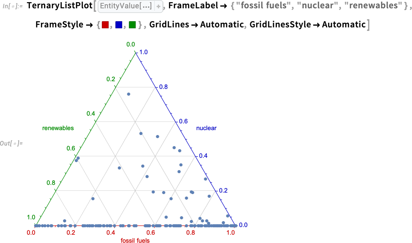
The plot shows the “energy mixture” for different countries, with the ones on the bottom axis being those with zero nuclear. Inserting colors for each axis, along with grid lines, helps explain how to read the plot:

Most of the time plots are plotting numbers, or at least quantities. In Version 13.0, we extended functions like ListPlot to also accept dates. In Version 13.1 we’re going much further, and introducing the possibility of plotting what amount to purely symbolic values.

Let’s say our data consists of letters A through C:

How do we plot these? In Version 13.1 we just specify an ordinal scale:

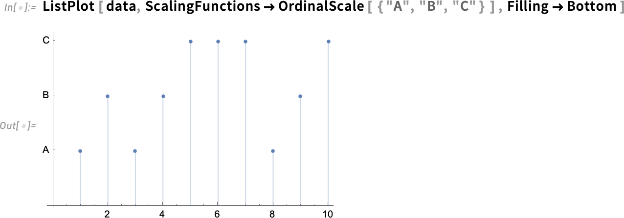
OrdinalScale lets you specify that certain symbolic values are to be treated as if they are in a specified order. There’s also the concept of a nominal scale—represented by NominalScale—in which different symbolic values correspond to different “categories”, but in no particular order.

New Aesthetics

Graphics: More Beautiful & Alive (January 2024)

Graphics have always been an important part of the story of the Wolfram Language, and for more than three decades we’ve been progressively enhancing and updating their appearance and functionality—sometimes with help from advances in hardware (e.g. GPU) capabilities.

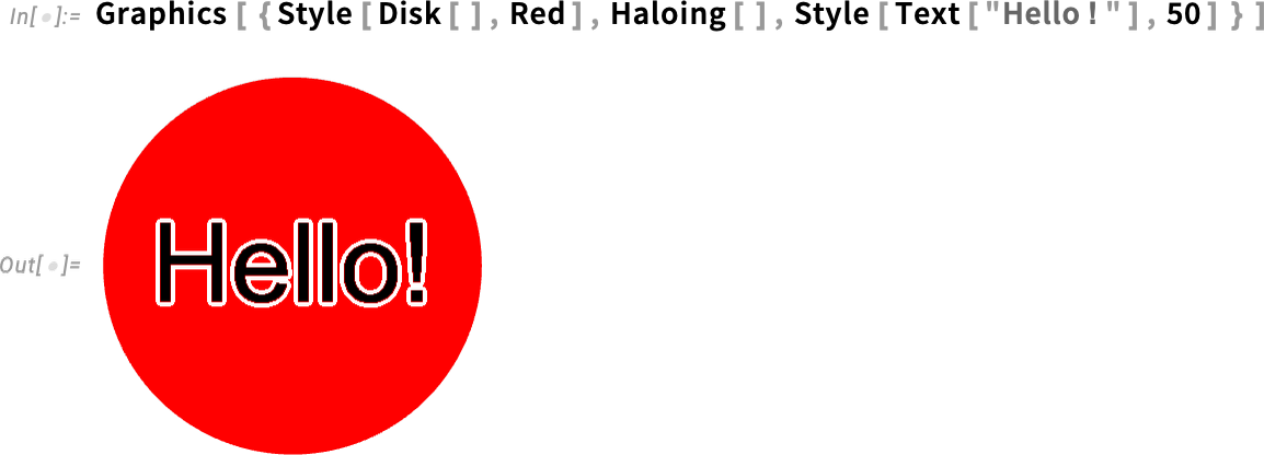
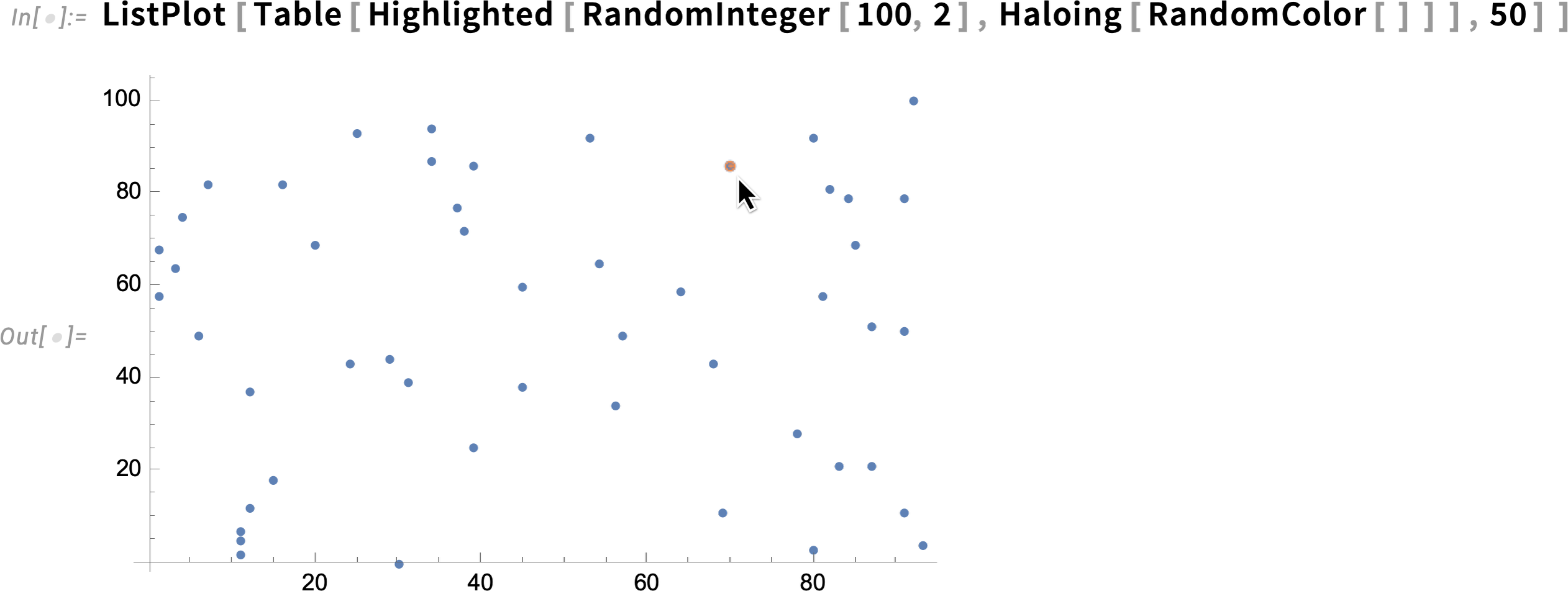
Since Version 13 we’ve added a variety of “decorative” (or “annotative”) effects in 2D graphics. One example (useful for putting captions on things) is Haloing:

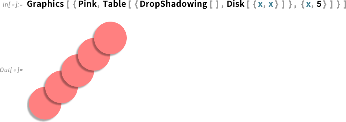
Another example is DropShadowing:

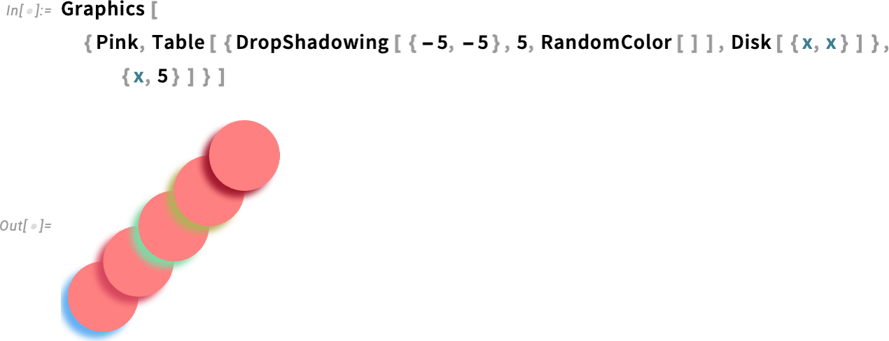
All of these are specified symbolically, and can be used throughout the system (e.g. in hover effects, etc). And, yes, there are many detailed parameters you can set:

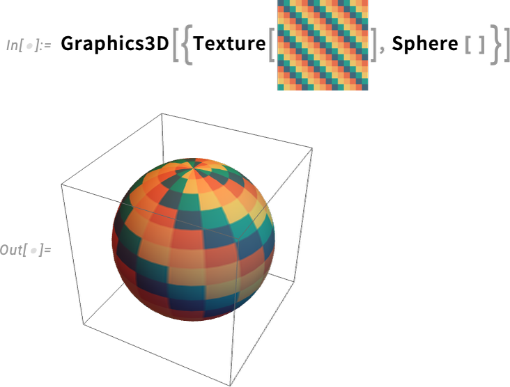
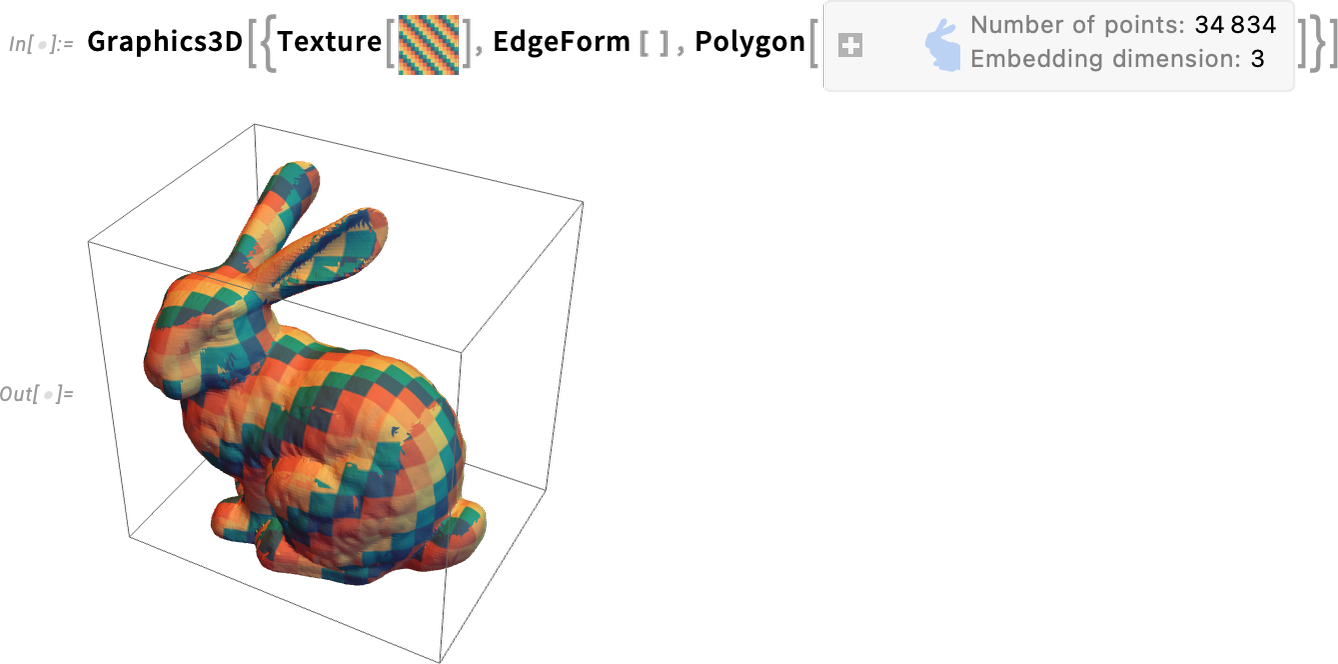
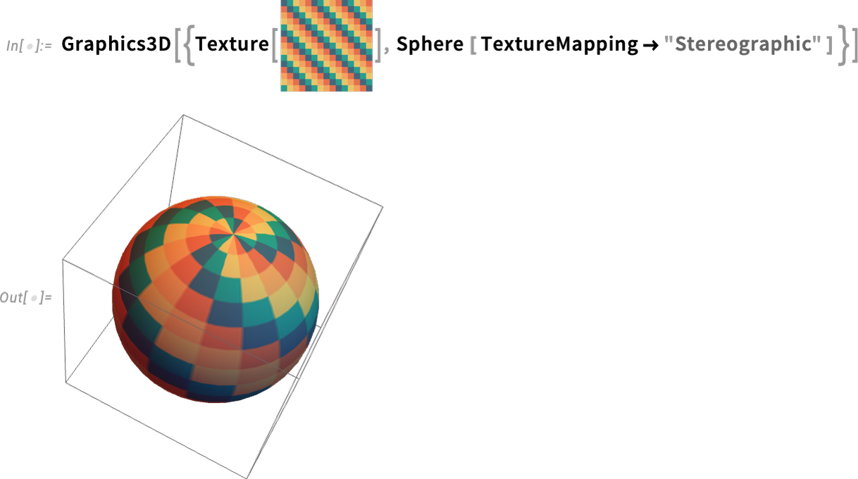
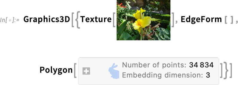
A significant new capability in Version 14.0 is convenient texture mapping. We’ve had low-level polygon-by-polygon textures for a decade and a half. But now in Version 14.0 we’ve made it straightforward to map textures onto whole surfaces. Here’s an example wrapping a texture onto a sphere:

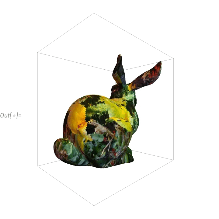
And here’s wrapping the same texture onto a more complicated surface:

A significant subtlety is that there are many ways to map what amount to “texture coordinate patches” onto surfaces. The documentation illustrates new, named cases:

And now here’s what happens with stereographic projection onto a sphere:

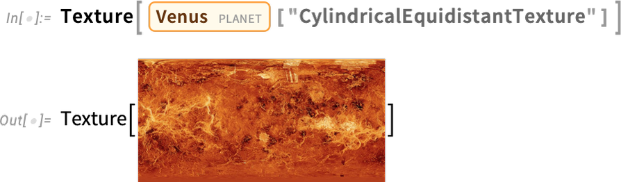
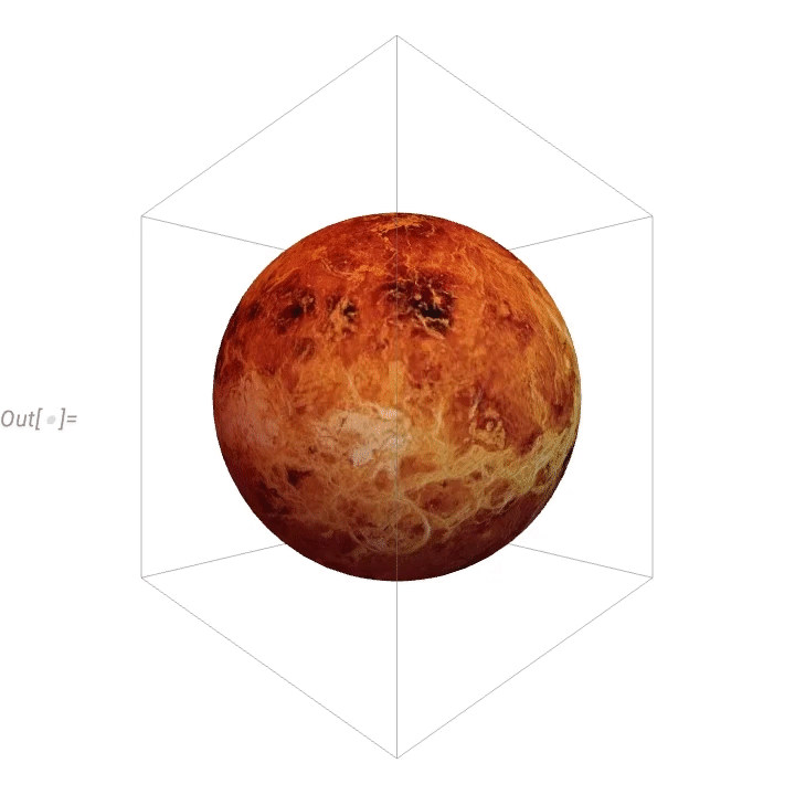
Here’s an example of “surface texture” for the planet Venus

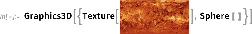
and here it’s been mapped onto a sphere, which can be rotated:

Here’s a “flowerified” bunny:

Things like texture mapping help make graphics visually compelling. Since Version 13 we’ve also added a variety of “live visualization” capabilities that automatically “bring visualizations to life”. For example, any plot now by default has a “coordinate mouseover”:

As usual, there’s lots of ways to control such “highlighting” effects:

Visual Effects & Beautification (June 2022)

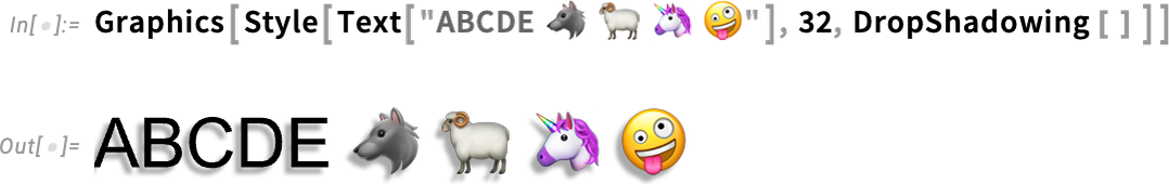
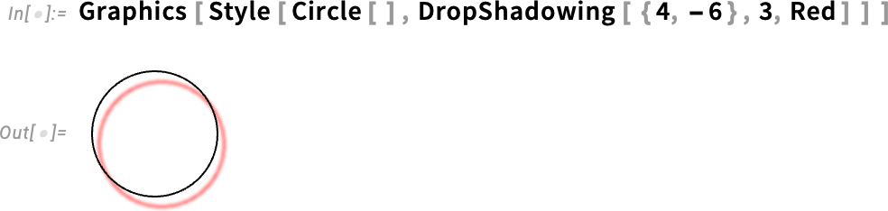
At first it seemed like a minor feature. But once we’d implemented it, we realized it was much more useful than we’d expected. Just as you can style a graphics object with its color (and, as of Version 13.0, its filling pattern), now in Version 13.1 you can style it with its drop shadowing:

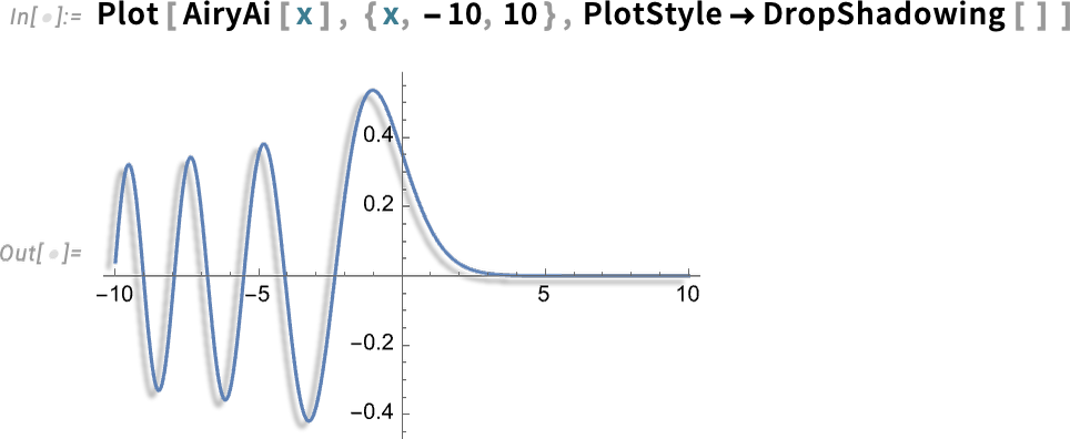
Drop shadowing turns out to be a nice way to “bring graphics to life”

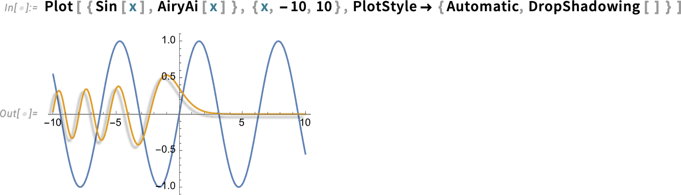
or to emphasize one element over others:

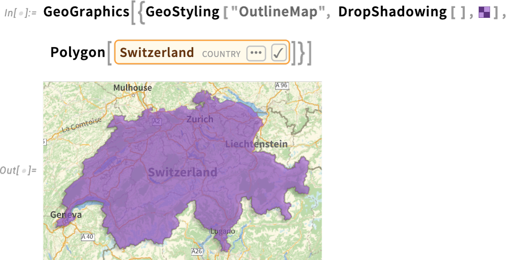
It works well in geo graphics as well:

DropShadowing allows detailed control over the shadows: what direction they’re in, how blurred they are and what color they are:

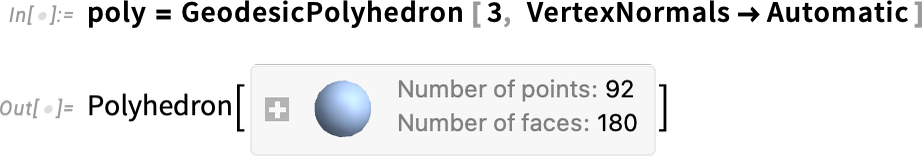
Drop shadowing is more complicated “under the hood” than one might imagine. And when possible it actually works using hardware GPU pixel shaders—the same technology that we’ve used since Version 12.3 to implement material-based surface textures for 3D graphics. In Version 13.1 we’ve explicitly exposed some well-known underlying types of 3D shading. Here’s a geodesic polyhedron (yes, that’s another new function in Version 13.1), with its surface normals added (using the again new function EstimatedPointNormals):

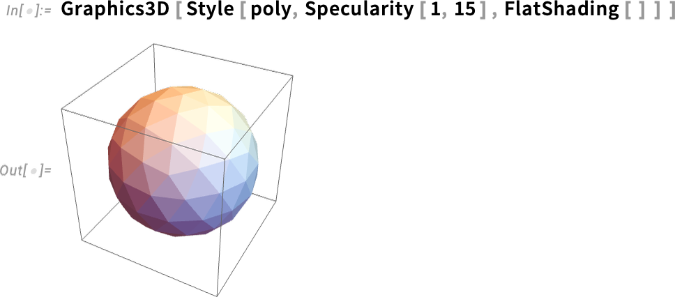
Here’s the most basic form of shading: flat shading of each facet (and the specularity in this case doesn’t “catch” any facets):

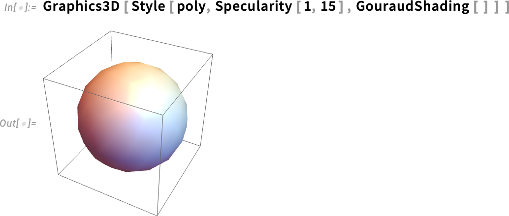
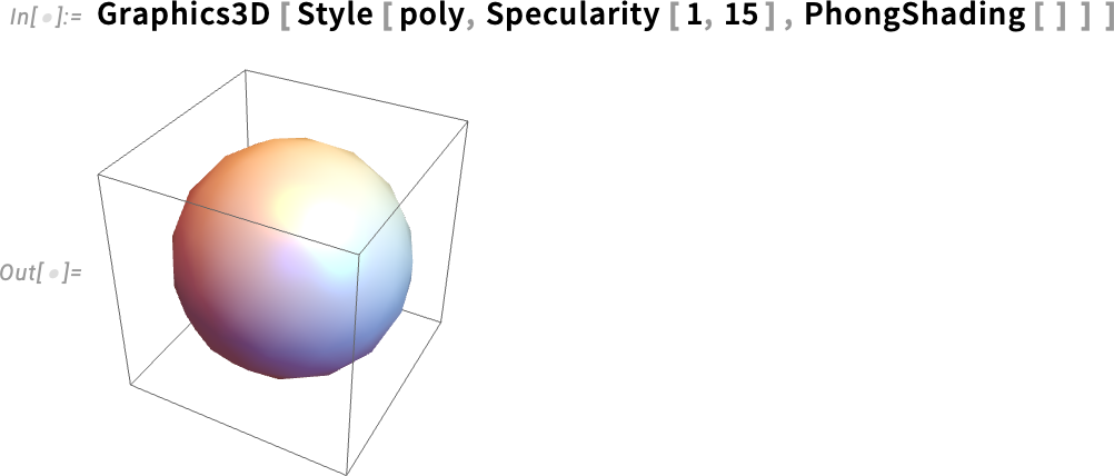
Here now is Gouraud shading, with a somewhat-faceted glint:

And then there’s Phong shading, looking somewhat more natural for a sphere:

Ever since Version 1.0, we’ve had an interactive way to rotate—and zoom into—3D graphics. (Yes, the mechanism was a bit primitive 34 years ago, but it rapidly got to more or less its modern form.) But in Version 13.1 we’re adding something new: the ability to “dolly” into a 3D graphic, imitating what would happen if you actually walked into a physical version of the graphic, as opposed to just zooming your camera:

And, yes, things can get a bit surreal (or “treky”)—here dollying in and then zooming out:

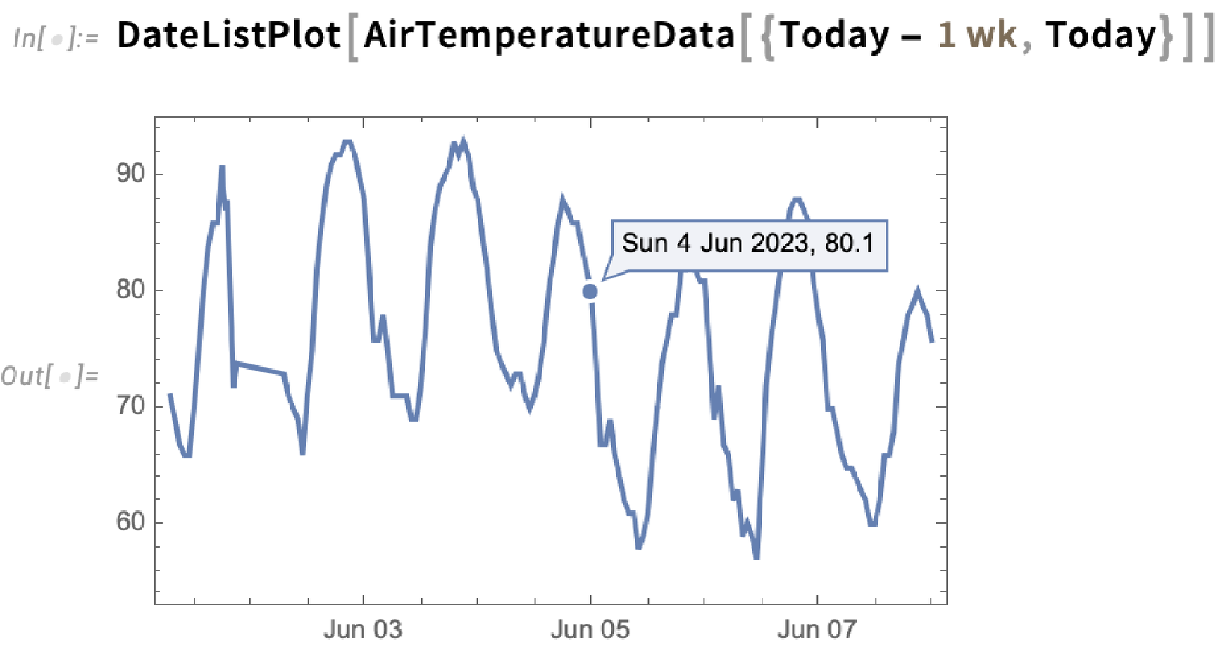
Visualizations Begin to Come Alive (June 2023)

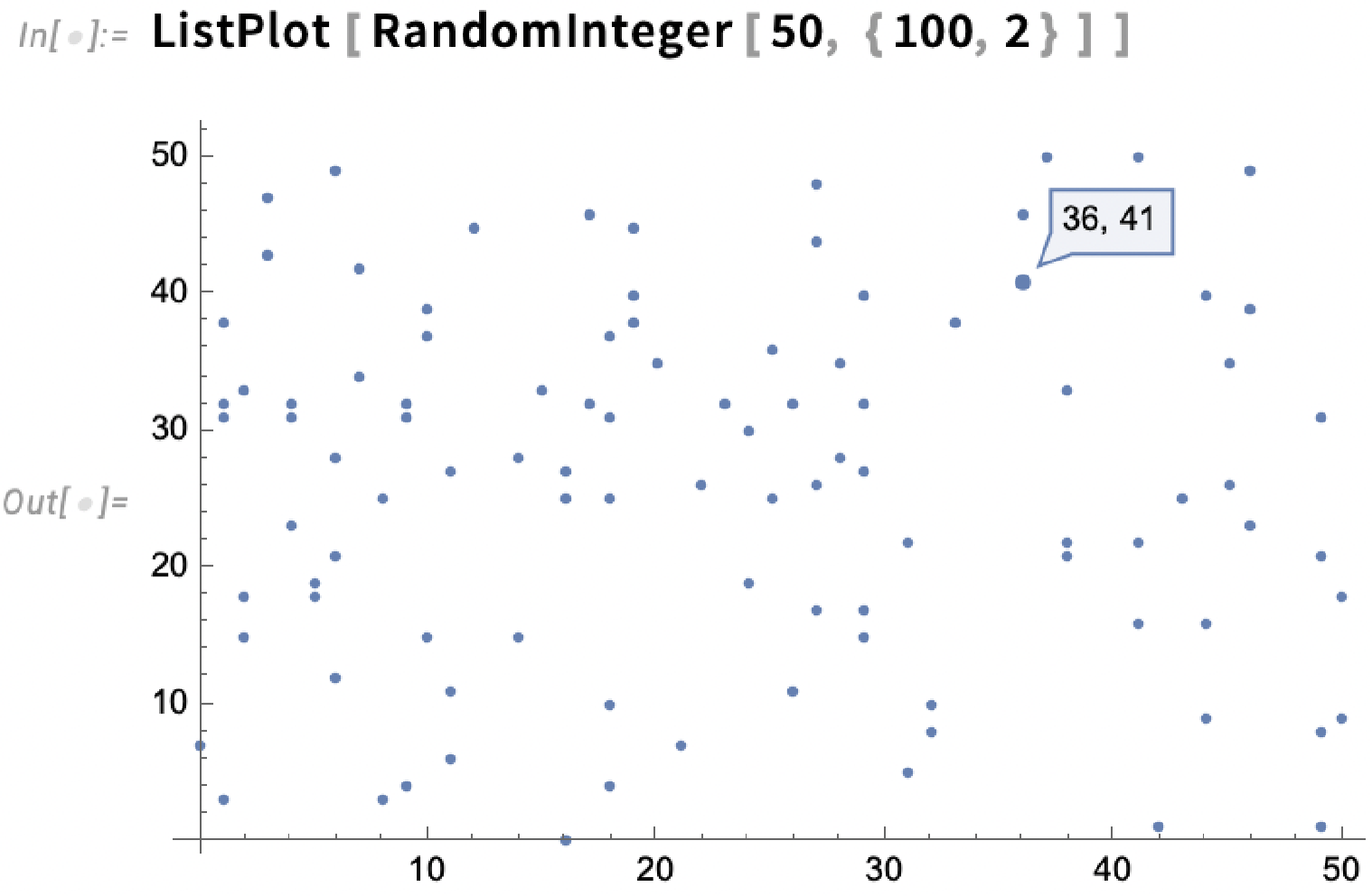
A great long-term strength of the Wolfram Language has been its ability to produce insightful visualizations in a highly automated way. In Version 13.3 we’re taking this further, by adding automatic “live highlighting”. Here’s a simple example, just using the function Plot. Instead of just producing static curves, Plot now automatically generates a visualization with interactive highlighting:

The same thing works for ListPlot:

The highlighting can, for example, show dates too:

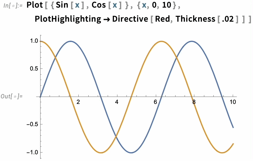
There are many choices for how the highlighting should be done. The simplest thing is just to specify a style in which to highlight whole curves:

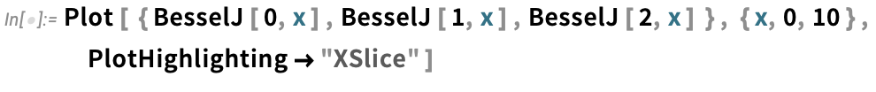
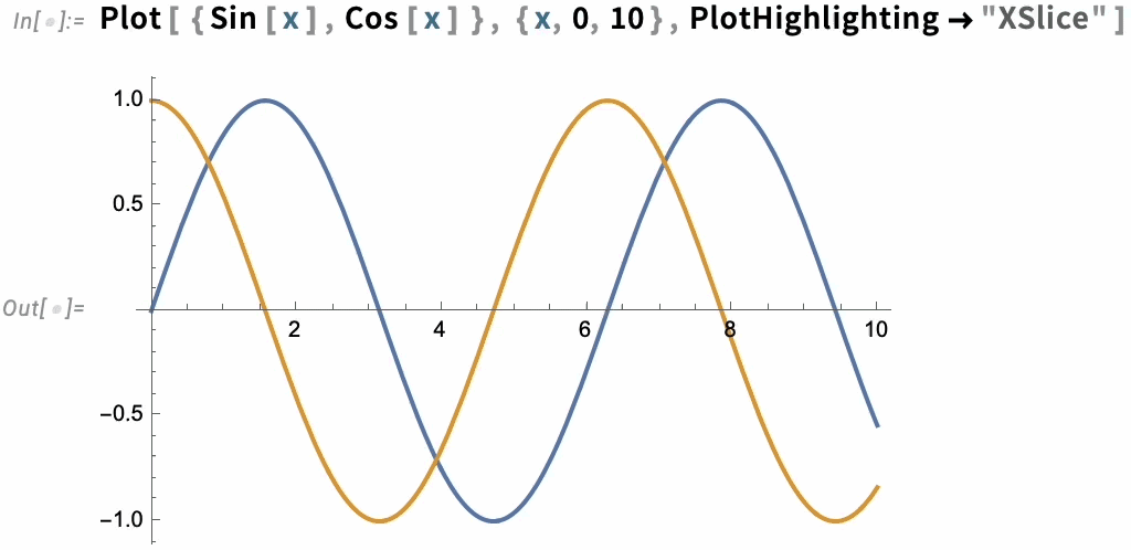
But there are many other built-in highlighting specifications. Here, for example, is "XSlice":

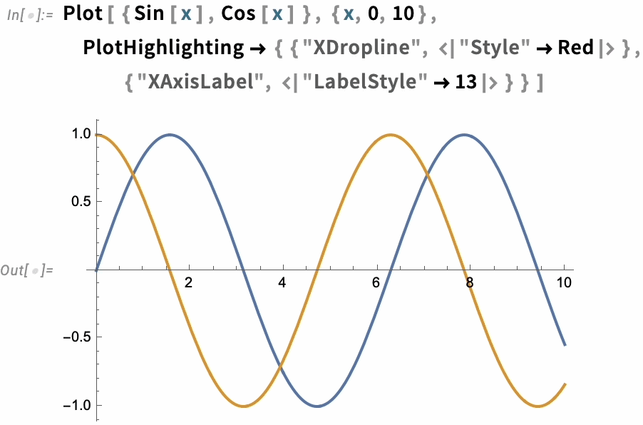
In the end, though, highlighting is built up from a whole collection of components—like "NearestPoint", "Crosshairs", "XDropline", etc.—that you can assemble and style for yourself:

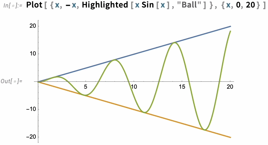
The option PlotHighlighting defines global highlighting in a plot. But by using the Highlighted “wrapper” you can specify that only a particular element in the plot should be highlighted:

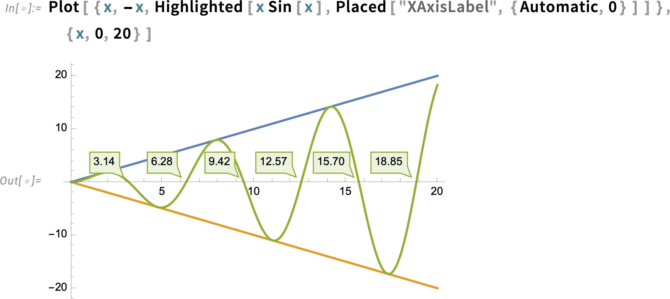
For interactive and exploratory purposes, the kind of automatic highlighting we’ve just been showing is very convenient. But if you’re making a static presentation, you’ll need to “burn in” particular pieces of highlighting—which you can do with Placed:

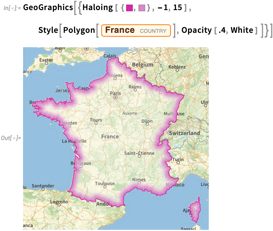
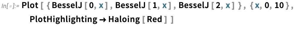
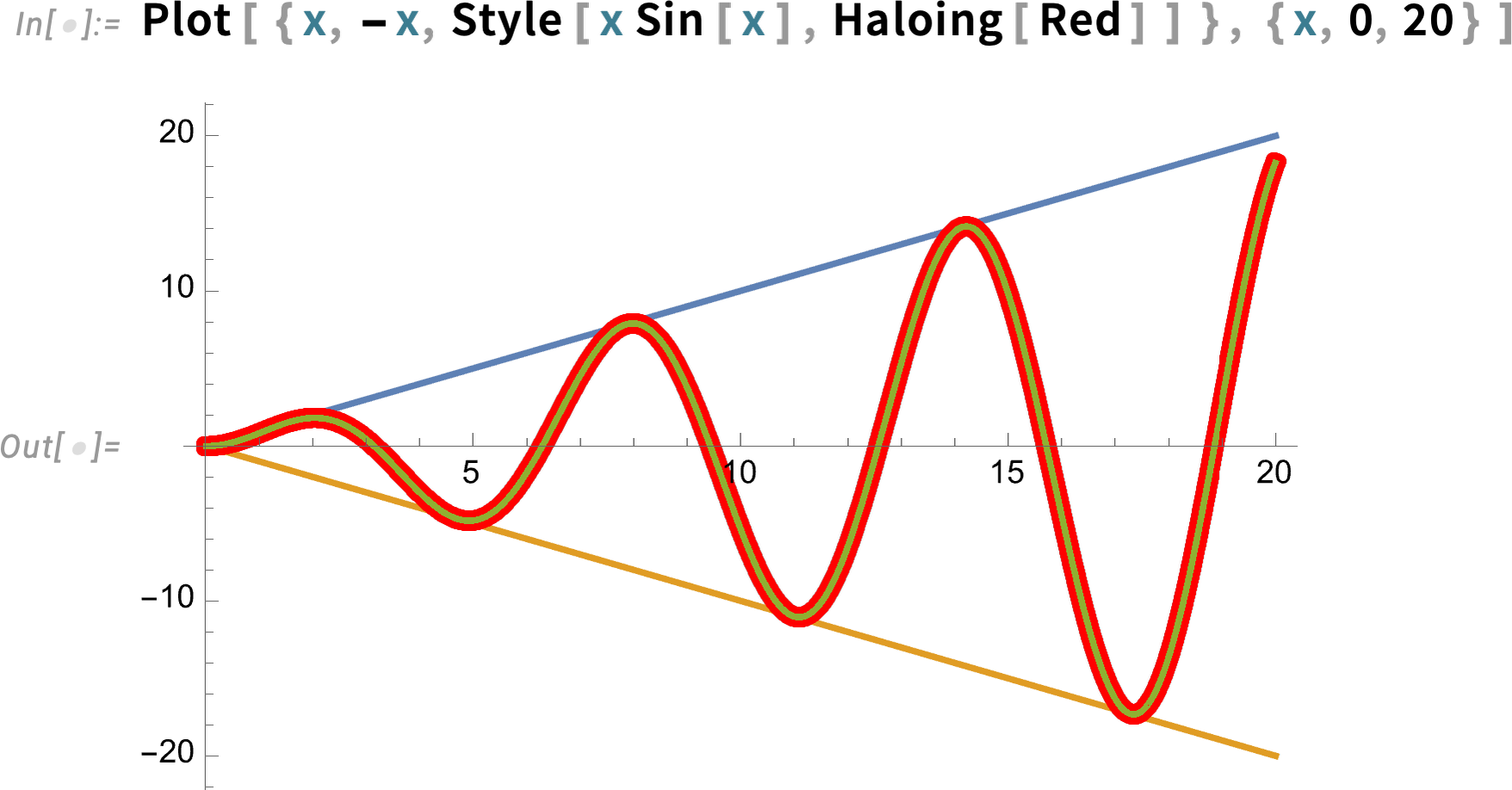
In indicating elements in a graphic there are different effects one can use. In Version 13.1 we introduced DropShadowing[]. In Version 13.3 we’re introducing Haloing:

Haloing can also be combined with interactive highlighting:

By the way, there are lots of nice effects you can get with Haloing in graphics. Here’s a geo example—including some parameters for the “orientation” and “thickness” of the haloing: