Two years ago we released Version 13.0 of Wolfram Language. Here are the updates in PDEs and system modeling since then, including the latest features in 14.0. The contents of this post are compiled from Stephen Wolfram’s Release Announcements for 13.1, 13.2, 13.3 and 14.0.

PDEs

Industrial-Strength Multidomain PDEs (January 2024)

PDEs are hard. It’s hard to solve them. And it’s hard to even specify what exactly you want to solve. But we’ve been on a multi-decade mission to “consumerize” PDEs and make them easier to work with. Many things go into this. You need to be able to easily specify elaborate geometries. You need to be able to easily define mathematically complicated boundary conditions. You need to have a streamlined way to set up the complicated equations that come out of underlying physics. Then you have to—as automatically as possible—do the sophisticated numerical analysis to efficiently solve the equations. But that’s not all. You also often need to visualize your solution, compute other things from it, or run optimizations of parameters over it.

It’s a deep use of what we’ve built with Wolfram Language—touching many parts of the system. And the result is something unique: a truly streamlined and integrated way to handle PDEs. One’s not dealing with some (usually very expensive) “just for PDEs” package; what we now have is a “consumerized” way to handle PDEs whenever they’re needed—for engineering, science, or whatever. And, yes, being able to connect machine learning, or image computation, or curated data, or data science, or real-time sensor feeds, or parallel computing, or, for that matter, Wolfram Notebooks, to PDEs just makes them so much more valuable.

We’ve had “basic, raw NDSolve” since 1991. But what’s taken decades to build is all the structure around that to let one conveniently set up—and efficiently solve—real-world PDEs, and connect them into everything else. It’s taken developing a whole tower of underlying algorithmic capabilities such as our more-flexible-and-integrated-than-ever-before industrial-strength computational geometry and finite element methods. But beyond that it’s taken creating a language for specifying real-world PDEs. And here the symbolic nature of the Wolfram Language—and our whole design framework—has made possible something very unique, that has allowed us to dramatically simplify and consumerize the use of PDEs.

It’s all about providing symbolic “construction kits” for PDEs and their boundary conditions. We started this about five years ago, progressively covering more and more application areas. In Version 14 we’ve particularly focused on solid mechanics, fluid mechanics, electromagnetics and (one-particle) quantum mechanics.

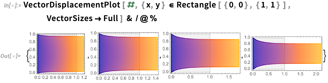
Here’s an example from solid mechanics. First, we define the variables we’re dealing with (displacement and underlying coordinates):

Next, we specify the parameters we want to use to describe the solid material we’re going to work with:

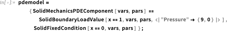
Now we can actually set up our PDE—using symbolic PDE specifications like SolidMechanicsPDEComponent—here for the deformation of a solid object pulled on one side:

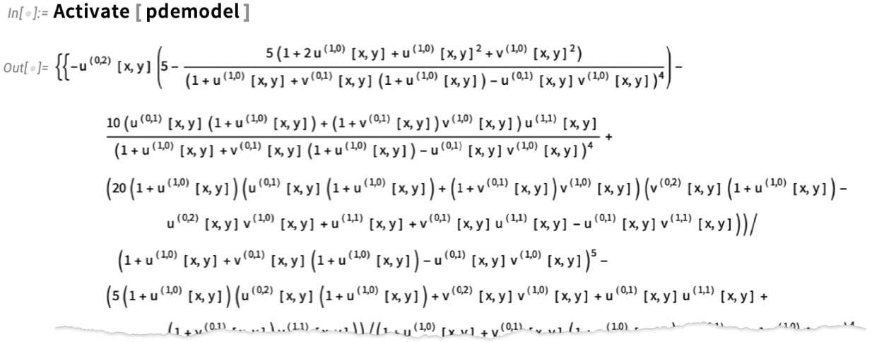
And, yes, “underneath”, these simple symbolic specifications turn into a complicated “raw” PDE:

Now we are ready to actually solve our PDE in a particular region, i.e. for an object with a particular shape:

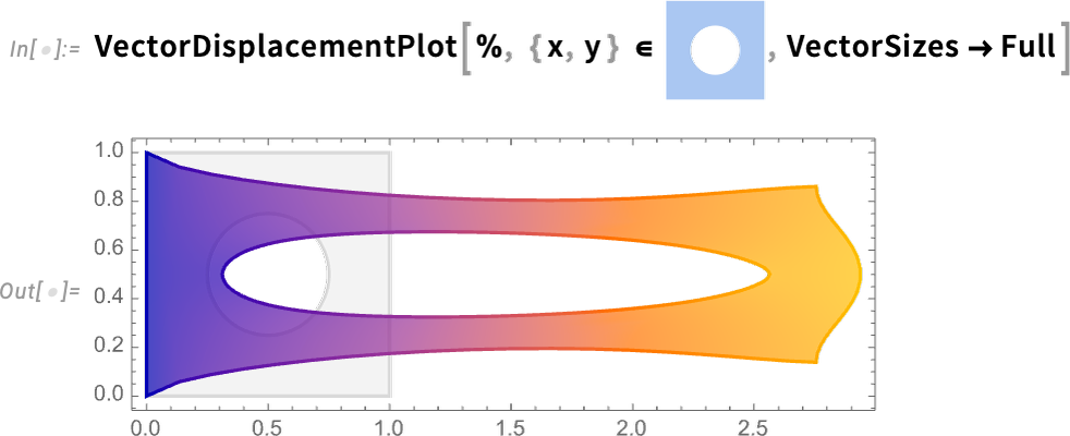
And now we can visualize the result, which shows how our object stretches when it’s pulled on:

The way we’ve set things up, the material for our object is an idealization of something like rubber. But in the Wolfram Language we now have ways to specify all sorts of detailed properties of materials. So, for example, we can add reinforcement as a unit vector in a particular direction (say in practice with fibers) to our material:

Then we can rerun what we did before

but now we get a slightly different result:

Another major PDE domain that’s new in Version 14.0 is fluid flow. Let’s do a 2D example. Our variables are 2D velocity and pressure:

Now we can set up our fluid system in a particular region, with no-slip conditions on all walls except at the top where we assume fluid is flowing from left to right. The only parameter needed is the Reynolds number. And instead of just solving our PDEs for a single Reynolds number, let’s create a parametric solver that can take any specified Reynolds number:

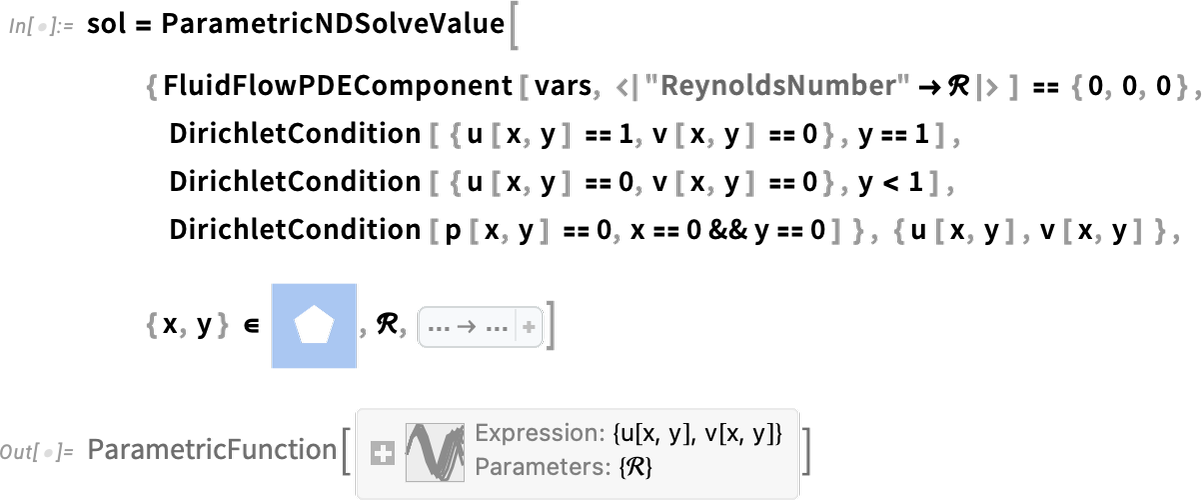
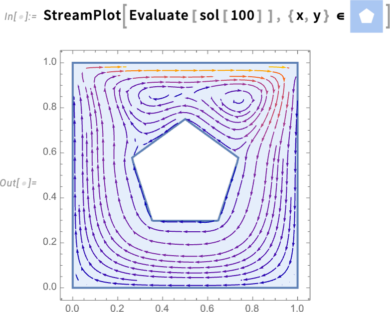
Now here’s the result for Reynolds number 100:

But with the way we’ve set things up, we can as well generate a whole video as a function of Reynolds number (and, yes, the Parallelize speeds things up by generating different frames in parallel):

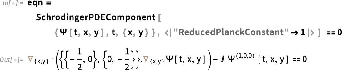
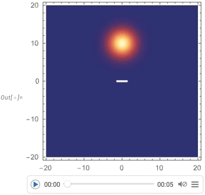
Much of our work in PDEs involves catering to the complexities of real-world engineering situations. But in Version 14.0 we’re also adding features to support “pure physics”, and in particular to support quantum mechanics done with the Schrödinger equation. So here, for example, is the 2D 1-particle Schrödinger equation (with ):

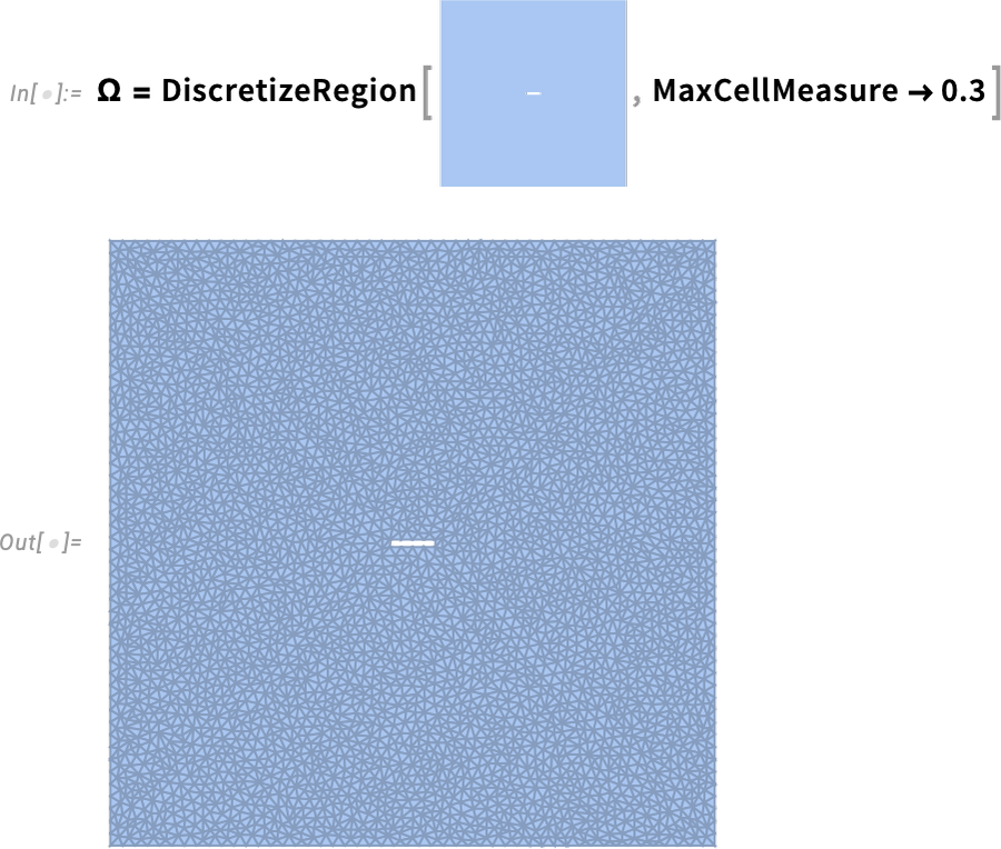
Here’s the region we’re going to be solving over—showing explicit discretization:

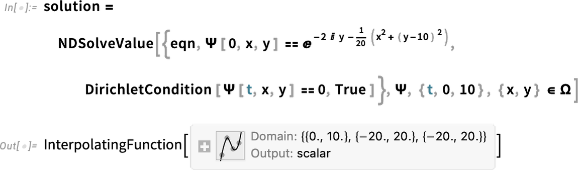
Now we can solve the equation, adding in some boundary conditions:

And now we get to visualize a Gaussian wave packet scattering around a barrier:

PDEs for Rods, Rubber and More (June 2022)

It’s been a 25-year journey, steadily increasing our built-in PDE capabilities. And in Version 13.1 we’ve added several (admittedly somewhat technical) features that have been much requested, and are important for solving particular kinds of real-world PDE problems. The first feature is being able to set up a PDE as axisymmetric. Normally a 2D diffusion term would be assumed Cartesian:

But now you can say you’re dealing with an axisymmetric system, with your coordinates being interpreted as radius and height, and everything assumed to be symmetrical in the azimuthal direction:

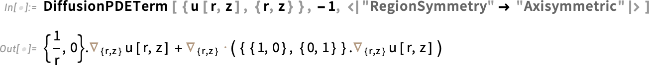
What’s important about this is not just that it makes it easy to set up certain kinds of equations, but also that in solving equations axial symmetry can be assumed, allowing much more efficient methods to be used:

Also in Version 13.1 is an extension to the solid mechanics modeling framework introduced in Version 13.0. Just as there’s viscosity that damps out motion in fluids, so there’s a similar phenomenon that damps out motion in solids. It’s more of an engineering story, and it’s usually described in terms of two parameters: mass damping and stiffness damping. And now in Version 13.1 we support this kind of so-called Rayleigh damping in our modeling framework.

Another phenomenon included in Version 13.1 is hyperelasticity. If you bend something like metal beyond a certain point (but not so far that it breaks), it’ll stay bent. But materials like rubber and foam (and some biological tissues) can “bounce back” from basically any deformation.

Let’s imagine that we have a square of rubber-like material. We anchor it on the left, and then we pull it on the right with a certain force. What does it do?

This defines the properties of our material:

We define variables for the problem, representing x and y displacements by u and v:

Now we can set up our whole problem, and solve the PDEs for it for each value of the force:

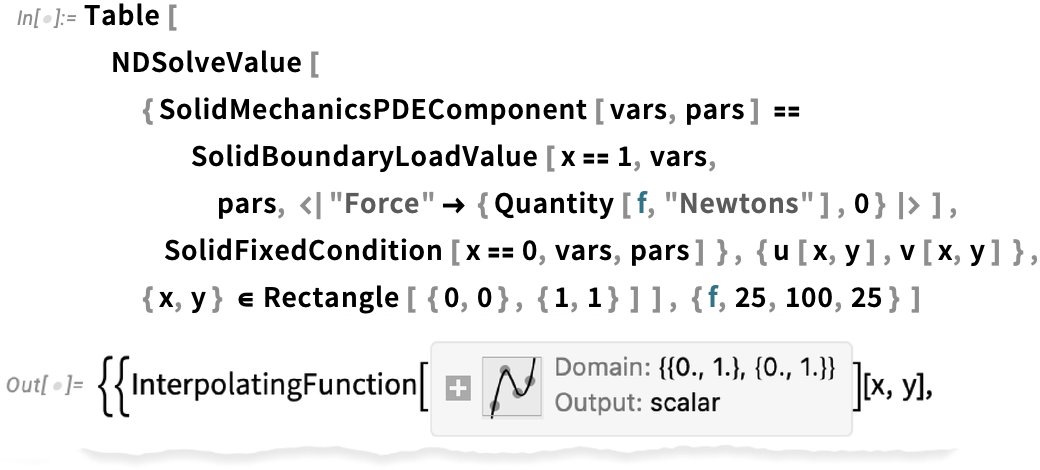
Then one can plot the results, and see the rubber being nonlinearly stretched:

There’s in the end considerable depth in our handling of PDE-based modeling, and our increasing ability to do “multiphysics” computations that span multiple types of physics (mechanical, thermal, electromagnetic, acoustic, …). And by now we’ve got nearly 1000 pages of documentation purely about PDE-based modeling. And for example in Version 13.1 we’ve added a monograph specifically about hyperelasticity, as well as expanded our collection of documented PDE models:

Control Systems

Streamlining Systems Engineering Computation 14 (January 2024)

Systems engineering is a big field, but it’s one where the structure and capabilities of the Wolfram Language provide unique advantages—that over the past decade have allowed us to build out rather complete industrial-strength support for modeling, analysis and control design for a wide range of types of systems. It’s all an integrated part of the Wolfram Language, accessible through the computational and interface structure of the language. But it’s also integrated with our separate Wolfram System Modeler product, that provides a GUI-based workflow for system modeling and exploration.

Shared with System Modeler are large collections of domain-specific modeling libraries. And, for example, since Version 13, we’ve added libraries in areas such as battery engineering, hydraulic engineering and aircraft engineering—as well as educational libraries for mechanical engineering, thermal engineering, digital electronics, and biology. (We’ve also added libraries for areas such as business and public policy simulation.)

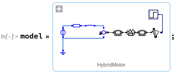
A typical workflow for systems engineering begins with the setting up of a model. The model can be built from scratch, or assembled from components in model libraries—either visually in Wolfram System Modeler, or programmatically in the Wolfram Language. For example, here’s a model of an electric motor that’s turning a load through a flexible shaft:

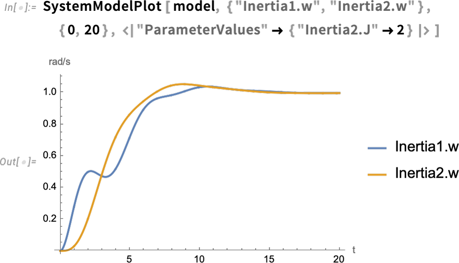
Once one’s got a model, one can then simulate it. Here’s an example where we’ve set one parameter of our model (the moment of inertia of the load), and we’re computing the values of two others as a function of time:

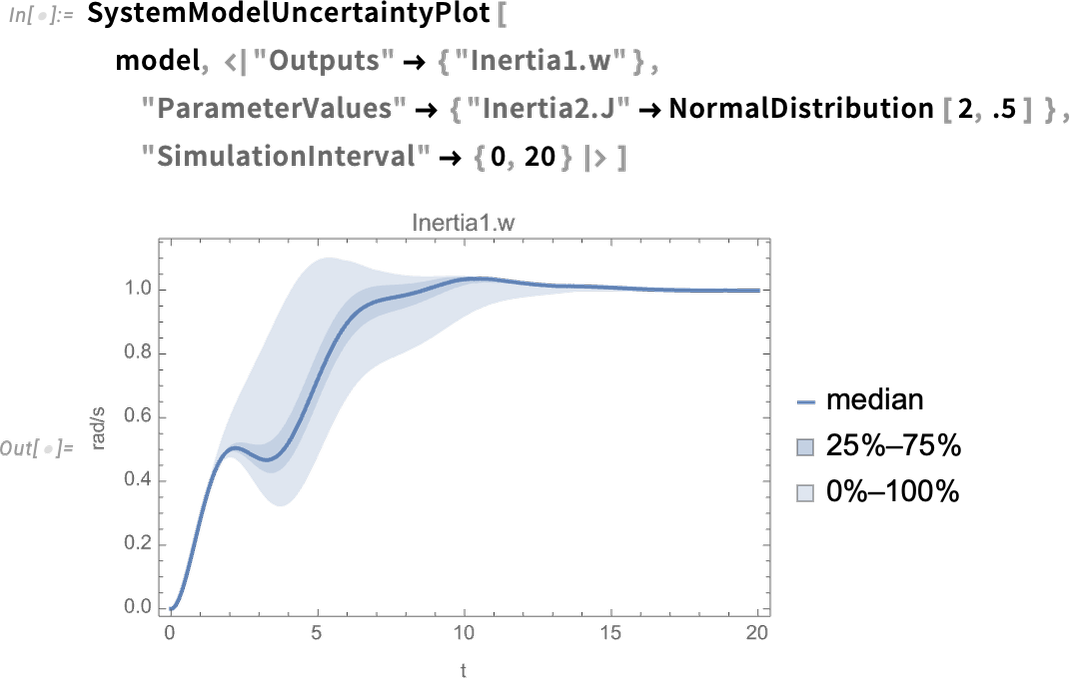
A new capability in Version 14.0 is being able to see the effect of uncertainty in parameters (or initial values, etc.) on the behavior of a system. So here, as an example, we’re saying the value of the parameter is not definite, but is instead distributed according to a normal distribution—then we’re seeing the distribution of output results:

The motor with flexible shaft that we’re looking at can be thought of as a “multidomain system”, combining electrical and mechanical components. But the Wolfram Language (and Wolfram System Modeler) can also handle “mixed systems”, combining analog and digital (i.e. continuous and discrete) components. Here’s a fairly sophisticated example from the world of control systems: a helicopter model connected in a closed loop to a digital control system:

This whole model system can be represented symbolically just by:

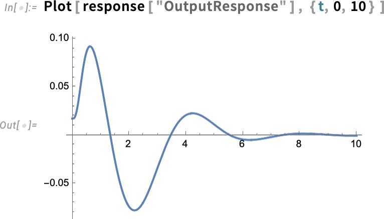
And now we compute the input-output response of the model:

Here’s specifically the output response:

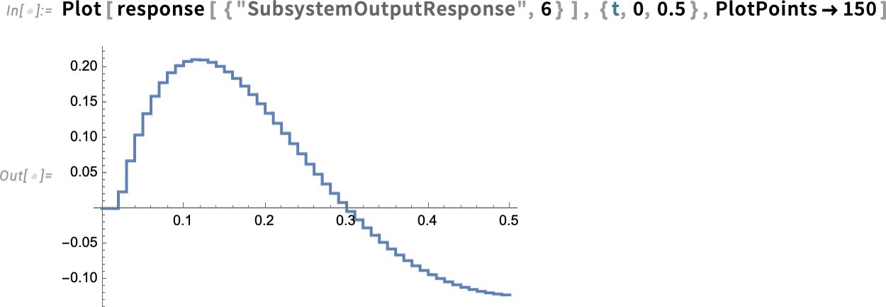
But now we can “drill in” and see specific subsystem responses, here of the zero-order hold device (labeled ZOH above)—complete with its little digital steps:

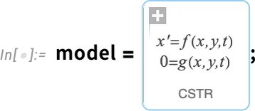
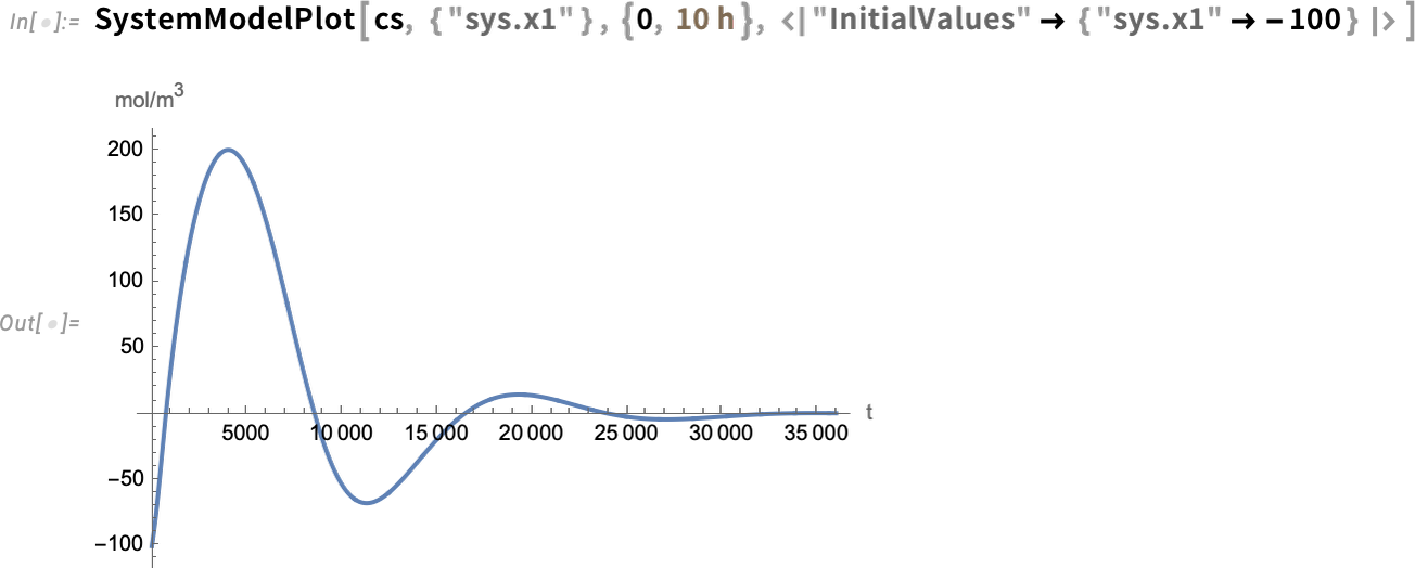
But what if we want to design the control systems ourselves? Well, in Version 14 we can now apply all our Wolfram Language control systems design functionality to arbitrary system models. Here’s an example of a simple model, in this case in chemical engineering (a continuously stirred tank):

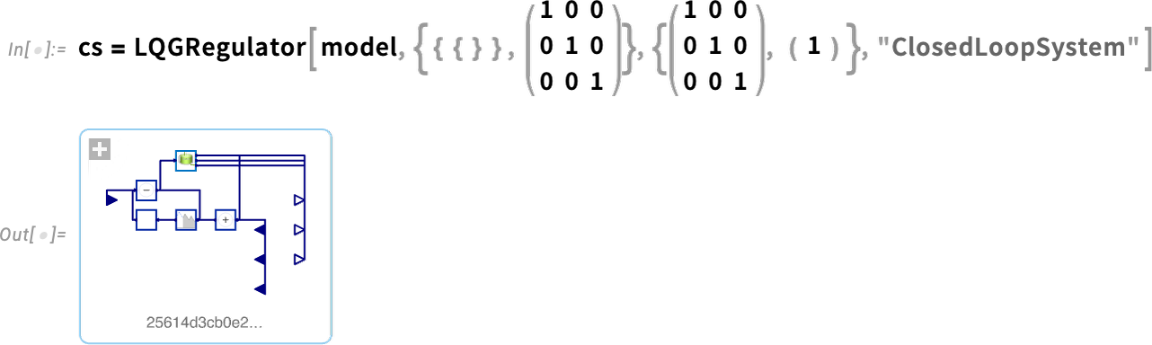
Now we can take this model and design an LQG controller for it—then assemble a whole closed-loop system for it:

Now we can simulate the closed-loop system—and see that the controller succeeds in bringing the final value to 0:

Model Predictive Control (June 2022)

One area that leverages many algorithmic capabilities of the Wolfram Language is control systems. We first started developing control systems functionality more than 25 years ago, and by Version 8.0 ten years ago we started to have built-in functions like StateSpaceModel and BodePlot specifically for working with control systems.

Over the past decade we’ve progressively been adding more built-in control systems capabilities, and in Version 13.1 we’re now introducing model predictive controllers (MPCs). Many simple control systems (like PID controllers) take an ad hoc approach in which they effectively just “watch what a system does” without trying to have a specific model for what’s going on inside the system. Model predictive control is about having a specific model for a system, and then deriving an optimal controller based on that model.

For example, we could have a state-space model for a system:

&#10005

Then in Version 13.1 we can derive (using our parametric optimization capabilities) an optimal controller that minimizes a certain set of costs while satisfying particular constraints:

&#10005

The SystemsModelControllerData that we get here contains a variety of elements that allow us to automate the control design and analysis workflow. As an example, we can get a model that represents the controller running in a closed loop with the system it is controlling:

&#10005

Now let’s imagine that we drive this whole system with the input:

&#10005

Now we can compute the output response for the system, and we see that both output variables are driven to zero through the operation of the controller:

&#10005

Within the SystemsModelControllerData object generated by ModelPredictiveController is the actual controller computed in this case—using the new construct DiscreteInputOutputModel:

&#10005

What actually is this controller? Ultimately it’s a collection of piecewise functions that depends on the values of states x₁[t] and x₂[t]:

&#10005

And this shows the different state-space regions in which the controller has:

&#10005

Digital Twins: Fitting System Models to Data (June 2023)

It’s been five years since we first began to introduce industrial-scale systems engineering capabilities in the Wolfram Language. The goal is to be able to compute with models of engineering and other systems that can be described by (potentially very large) collections of ordinary differential equations and their discrete analogs. Our separate Wolfram System Modeler product provides an IDE and GUI for graphically creating such models.

For the past five years we’ve been able to do high-efficiency simulation of these models from within the Wolfram Language. And over the past few years we’ve been adding all sorts of higher-level functionality for programmatically creating models, and for systematically analyzing their behavior. A major focus in recent versions has been the synthesis of control systems, and various forms of controllers.

Version 13.3 now tackles a different issue, which is the alignment of models with real-world systems. The idea is to have a model which contains certain parameters, and then to determine these parameters by essentially fitting the model’s behavior to observed behavior of a real-world system.

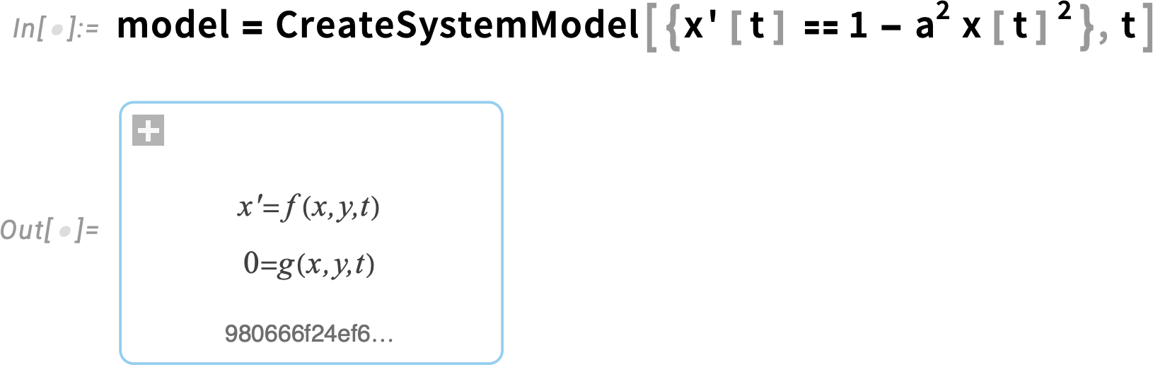
Let’s start by talking about a simple case where our model is just defined by a single ODE:

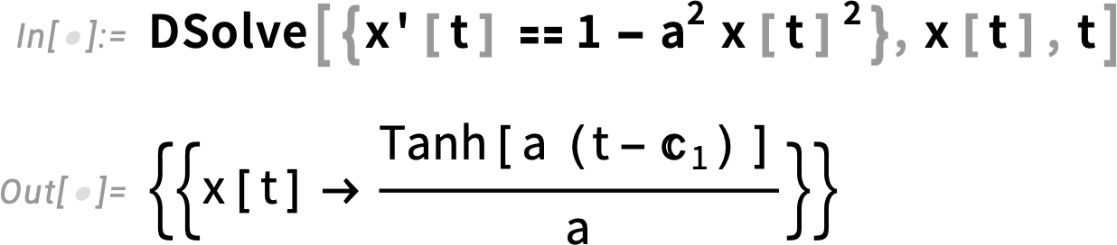
This ODE is simple enough that we can find its analytical solution:

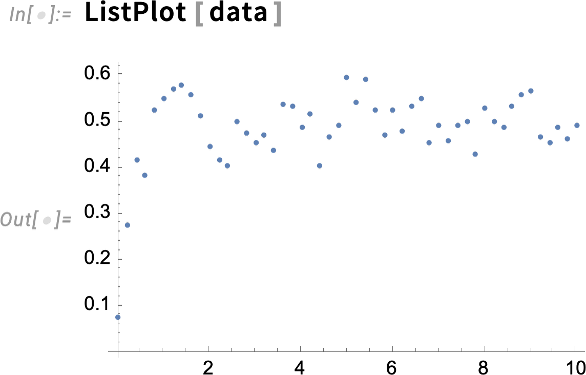
So now let’s make some “simulated real-world data” assuming a = 2, and with some noise:

Here’s what the data looks like:

Now let’s try to “calibrate” our original model using this data. It’s a process similar to machine learning training. In this case we make an “initial guess” that the parameter a is 1; then when SystemModelCalibrate runs it shows the “loss” decreasing as the correct value of a is found:

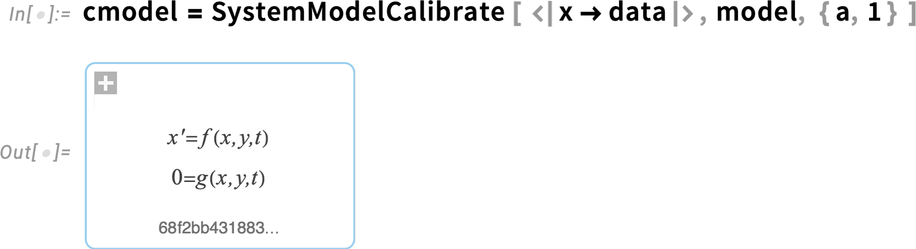
The “calibrated” model does indeed have a ≈ 2:

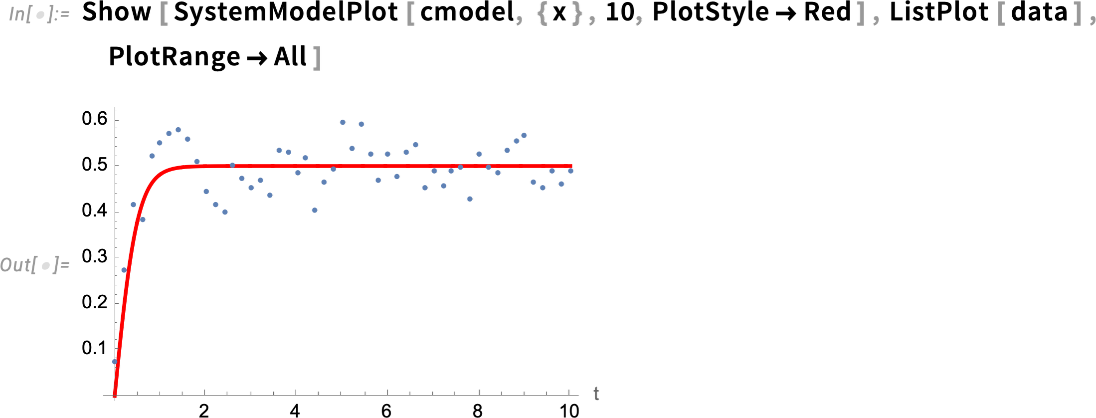
Now we can compare the calibrated model with the data:

As a slightly more realistic engineering-style example let’s look at a model of an electric motor (with both electrical and mechanical parts):

Let’s say we’ve got some data on the behavior of the motor; here we’ve assumed that we’ve measured the angular velocity of a component in the motor as a function of time. Now we can use this data to calibrate parameters of the model (here the resistance of a resistor and the damping constant of a damper):

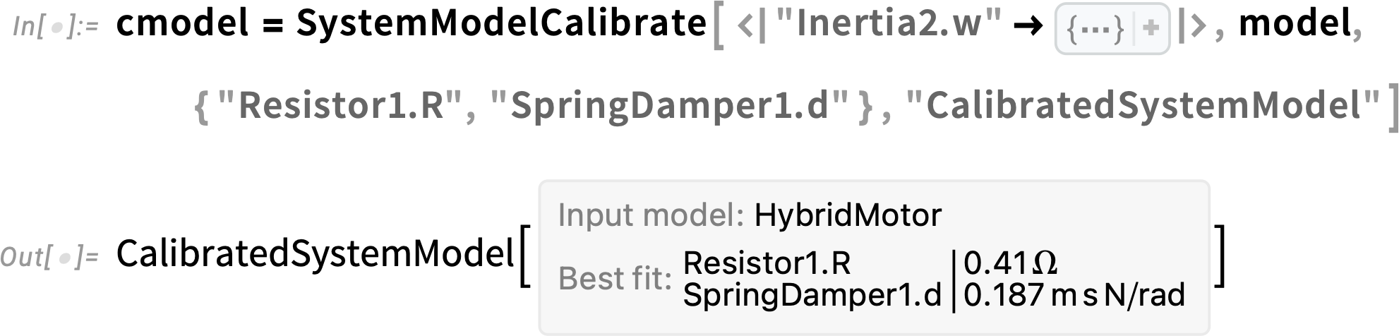
Here are the fitted parameter values:

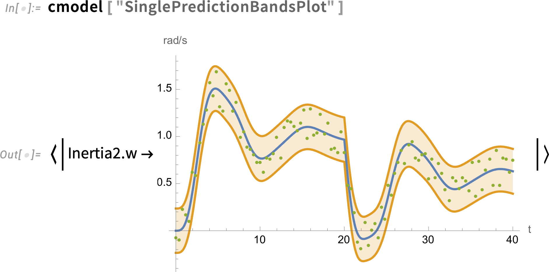
And here’s a full plot of the angular velocity data, together with the fitted model and its 95% confidence bands:

SystemModelCalibrate can be used not only in fitting a model to real-world data, but also for example in fitting simpler models to more complicated ones, making possible various forms of “model simplification”.