Two years ago we released Version 13.0 of Wolfram Language. Here are the updates in video since then, including the latest features in 14.0. The contents of this post are compiled from Stephen Wolfram’s Release Announcements for 13.1, 13.2, 13.3 and 14.0.

Quizzes & Assessments

Algorithmic and Randomized Quizzes (June 2022)

In Version 13.0 we introduced our question and assessment framework that allows you to author things like quizzes in notebooks, together with assessment functions, then deploy these for use. In Version 13.1 we’re adding capabilities to let you algorithmically or randomly generate questions.

The two new functions QuestionGenerator and QuestionSelector let you specify questions to be generated according to a template, or randomly selected from a pool. You can either use these functions directly in pure Wolfram Language code, or you can use them through the Question Notebook authoring GUI.

When you select Insert Question in the GUI, you now get a choice between Fixed Question, Randomized Question and Generated Question:

&#10005

Pick Randomized Question and you’ll get

&#10005

which then allows you to enter questions, and eventually produce a QuestionSelector—which will select newly randomized questions for every copy of the quiz that’s produced:

&#10005

Version 13.1 also introduces some enhancements for authoring questions. An example is a pure-GUI “no-code” way to specify multiple-choice questions:

&#10005

Did You Get That Math Right? (June 2023)

Most of what the Wolfram Language is about is taking inputs from humans (as well as programs, and now AIs) and computing outputs from them. But a few years ago we started introducing capabilities for having the Wolfram Language ask questions of humans, and then assessing their answers.

In recent versions we’ve been building up sophisticated ways to construct and deploy “quizzes” and other collections of questions. But one of the core issues is always how to determine whether a person has answered a particular question correctly. Sometimes that’s easy to determine. If we ask “What is 2 + 2?”, the answer better be “4” (or conceivably “four”). But what if we ask a question where the answer is some algebraic expression? The issue is that there may be many mathematically equal forms of that expression. And it depends on what exactly one’s asking whether one considers a particular form to be the “right answer” or not.

For example, here we’re computing a derivative:

And here we’re doing a factoring problem:

These two answers are mathematically equal. And they’d both be “reasonable answers” for the derivative if it appeared as a question in a calculus course. But in an algebra course, one wouldn’t want to consider the unfactored form a “correct answer” to the factoring problem, even though it’s “mathematically equal”.

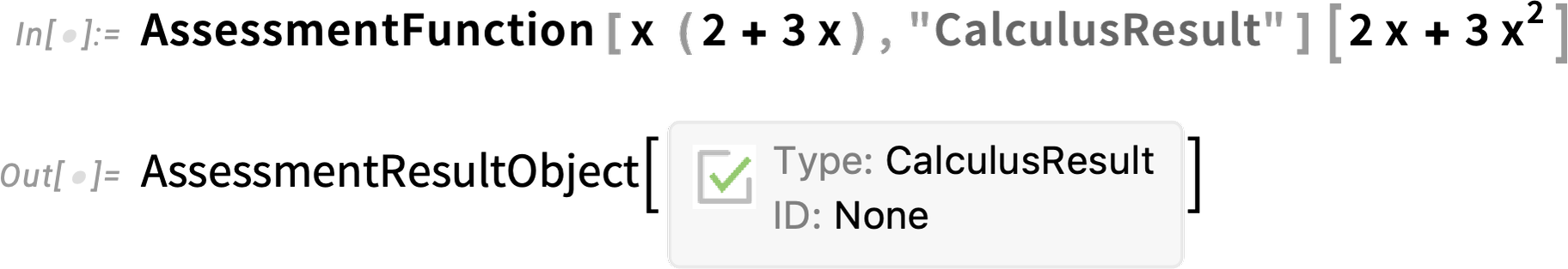
And to deal with these kinds of issues, we’re introducing in Version 13.3 more detailed mathematical assessment functions. With a "CalculusResult" assessment function, it’s OK to give the unfactored form:

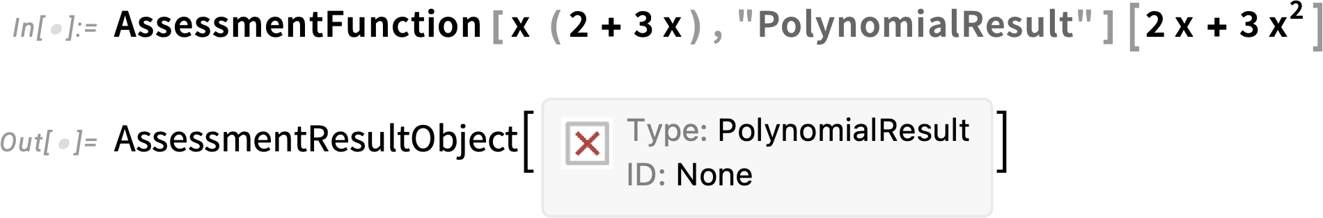
But with a "PolynomialResult" assessment function, the algebraic form of the expression has to be the same for it to be considered “correct”:

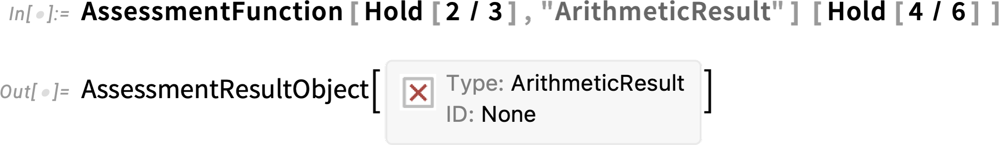
There’s also another type of assessment function—"ArithmeticResult"—which only allows trivial arithmetic rearrangements, so that it considers 2 + 3 equivalent to 3 + 2, but doesn’t consider 2/3 equivalent to 4/6:

Here’s how you’d build a question with this:

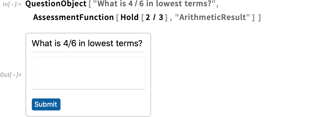
And now if you type “2/3” it’ll say you’ve got it right, but if you type “4/6” it won’t. However, if you use, say, "CalculusResult" in the assessment function, it’ll say you got it right even if you type “4/6”.

User Interface & Ease of Use

The Ever-Smoother User Interface (January 2024)

Our goal with Wolfram Language is to make it as easy as possible to express oneself computationally. And a big part of achieving that is the coherent design of the language itself. But there’s another part as well, which is being able to actually enter Wolfram Language input one wants—say in a notebook—as easily as possible. And with every new version we make enhancements to this.

One area that’s been in continuous development is interactive syntax highlighting. We first added syntax highlighting nearly two decades ago—and over time we’ve progressively made it more and more sophisticated, responding both as you type, and as code gets executed. Some highlighting has always had obvious meaning. But particularly highlighting that is dynamic and based on cursor position has sometimes been harder to interpret. And in Version 14—leveraging the brighter color palettes that have become the norm in recent years—we’ve tuned our dynamic highlighting so it’s easier to quickly tell “where you are” within the structure of an expression:

On the subject of “knowing what one has”, another enhancement—added in Version 13.2—is differentiated frame coloring for different kinds of visual objects in notebooks. Is that thing one has a graphic? Or an image? Or a graph? Now one can tell from the color of frame when one selects it:

An important aspect of the Wolfram Language is that the names of built-in functions are spelled out enough that it’s easy to tell what they do. But often the names are therefore necessarily quite long, and so it’s important to be able to autocomplete them when one’s typing. In 13.3 we added the notion of “fuzzy autocompletion” that not only “completes to the end” a name one’s typing, but also can fill in intermediate letters, change capitalization, etc. Thus, for example, just typing lll brings up an autocompletion menu that begins with ListLogLogPlot:

A major user interface update that first appeared in Version 13.1—and has been enhanced in subsequent versions—is a default toolbar for every notebook:

The toolbar provides immediate access to evaluation controls, cell formatting and various kinds of input (like inline cells, , hyperlinks, drawing canvas, etc.)—as well as to things like cloud publishing, documentation search and “chat” (i.e. LLM) settings.

Much of the time, it’s useful to have the toolbar displayed in any notebook you’re working with. But on the left-hand side there’s a little tiny that lets you minimize the toolbar:

In 14.0 there’s a Preferences setting that makes the toolbar come up minimized in any new notebook you create—and this in effect gives you the best of both worlds: you have immediate access to the toolbar, but your notebooks don’t have anything “extra” that might distract from their content.

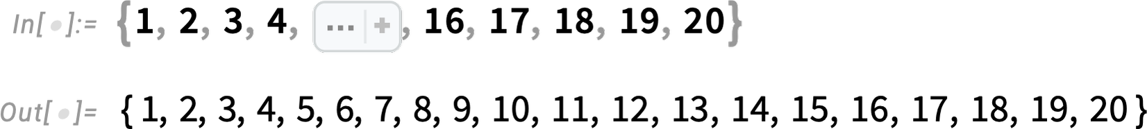
Another thing that’s advanced since Version 13 is the handling of “summary” forms of output in notebooks. A basic example is what happens if you generate a very large result. By default only a summary of the result is actually displayed. But now there’s a bar at the bottom that gives various options for how to handle the actual output:

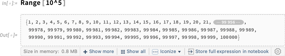
By default, the output is only stored in your current kernel session. But by pressing the Iconize button you get an iconized form that will appear directly in your notebook (or one that can be copied anywhere) and that “has the whole output inside”. There’s also a Store full expression in notebook button, which will “invisibly” store the output expression “behind” the summary display.

If the expression is stored in the notebook, then it’ll be persistent across kernel sessions. Otherwise, well, you won’t be able to get to it in a different kernel session; the only thing you’ll have is the summary display:

It’s a similar story for large “computational objects”. Like here’s a Nearest function with a million data points:

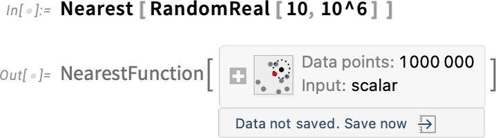
By default, the data is just something that exists in your current kernel session. But now there’s a menu that lets you save the data in various persistent locations:

And There’s the Cloud Too (January 2024)

There are many ways to run the Wolfram Language. Even in Version 1.0 we had the notion of remote kernels: the notebook front end running on one machine (in those days essentially always a Mac, or a NeXT), and the kernel running on a different machine (in those days sometimes even connected by phone lines). But a decade ago came a major step forward: the Wolfram Cloud.

There are really two distinct ways in which the cloud is used. The first is in delivering a notebook experience similar to our longtime desktop experience, but running purely in a browser. And the second is in delivering APIs and other programmatically accessed capabilities—notably, even at the beginning, a decade ago, through things like APIFunction.

The Wolfram Cloud has been the target of intense development now for nearly 15 years. Alongside it have also come Wolfram Application Server and Wolfram Web Engine, which provide more streamlined support specifically for APIs (without things like user management, etc., but with things like clustering).

All of these—but particularly the Wolfram Cloud—have become core technology capabilities for us, supporting many of our other activities. So, for example, the Wolfram Function Repository and Wolfram Paclet Repository are both based on the Wolfram Cloud (and in fact this is true of our whole resource system). And when we came to build the Wolfram plugin for ChatGPT earlier this year, using the Wolfram Cloud allowed us to have the plugin deployed within a matter of days.

Since Version 13 there have been quite a few very different applications of the Wolfram Cloud. One is for the function ARPublish, which takes 3D geometry and puts it in the Wolfram Cloud with appropriate metadata to allow phones to get augmented-reality versions from a QR code of a cloud URL:

On the Cloud Notebook side, there’s been a steady increase in usage, notably of embedded Cloud Notebooks, which have for example become common on Wolfram Community, and are used all over the Wolfram Demonstrations Project. Our goal all along has been to make Cloud Notebooks be as easy to use as simple webpages, but to have the depth of capabilities that we’ve developed in notebooks over the past 35 years. We achieved this some years ago for fairly small notebooks, but in the past couple of years we’ve been going progressively further in handling even multi-hundred-megabyte notebooks. It’s a complicated story of caching, refreshing—and dodging the vicissitudes of web browsers. But at this point the vast majority of notebooks can be seamlessly deployed to the cloud, and will display as immediately as simple webpages.

Emojis! And More Multilingual Support (June 2022)

What is a character? Back when Version 1.0 was released, characters were represented as 8-bit objects: usually ASCII, but you could pick another “character encoding” (hence the ChararacterEncoding option) if you wanted. Then in the early 1990s came Unicode—which we were one of the very first companies to support. Now “characters” could be 16-bit constructs, with nearly 65,536 possible “glyphs” allocated across different languages and uses (including some mathematical symbols that we introduced). Back in the early 1990s Unicode was a newfangled thing, that operating systems didn’t yet have built-in support for. But we were betting on Unicode, and so we built our own infrastructure for handling it.

Thirty years later Unicode is indeed the universal standard for representing character-like things. But somewhere along the way, it turned out the world needed more than 16 bits’ worth of character-like things. At first it was about supporting variants and historical writing systems (think: cuneiform or Linear B). But then came emoji. And it became clear that—yes, arguably in a return to the Egyptian hieroglyph style of communication—there was an almost infinite number of possible pictorial emoji that could be made, each of them being encoded as their own Unicode code point.

It’s been a slow expansion. Original 16-bit Unicode is “plane 0”. Now there are up to 16 additional planes. Not quite 32-bit characters, but given the way computers work, the approach now is to allow characters to be represented by 32-bit objects. It’s far from trivial to do that uniformly and efficiently. And for us it’s been a long process to upgrade everything in our system—from string manipulation to notebook rendering—to handle full 32-bit characters. And that’s finally been achieved in Version 13.1.

But that’s far from all. In English we’re pretty much used to being able to treat text as a sequence of letters and other characters, with each character being separate. Things get a bit more complicated when you start to worry about diphthongs like æ. But if there are fairly few of these, it works to just introduce them as individual “Unicode characters” with their own code point. But there are plenty of languages—like Hindi or Khmer—where what appears in text like an individual character is really a composite of letter-like constructs, diacritical marks and other things. Such composite characters are normally represented as “grapheme clusters”: runs of Unicode code points. The rules for handling these things can be quite complicated. But after many years of development, major operating systems now successfully do it in most cases. And in Version 13.1 we’re able to make use of this to support such constructs in notebooks.

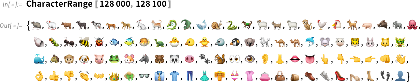
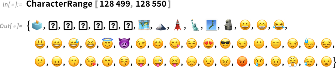
OK, so what does 32-bit Unicode look like? Using CharacterRange (or FromCharacterCode) we can dive in and just see what’s out there in “character space”. Here’s part of ordinary 16-bit Unicode space:

Here’s some of what happens in “plane-1” above character code 65535, in this case catering to “legacy computations”:

Plane-0 (below 65535) is pretty much all full. Above that, things are sparser. But around 128000, for example, there are lots of emoji:

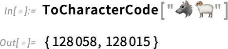
You can use these in the Wolfram Language, and in notebooks, just like any other characters. So, for example, you can have wolf and ram variables:

The 🐏 sorts before the 🐺 because it happens to have a numerically smaller character code:

In a notebook, you can enter emoji (and other Unicode characters) using standard operating system tools—like ctrlcmdspace on macOS:

&#10005

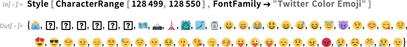
The world of emoji is rapidly evolving—and that can sometimes lead to problems. Here’s an emoji range that includes some very familiar emoji, but on at least one of my computer systems also includes emoji that display only as :

The reason that happens is that my default fonts don’t contain glyphs for those emoji. But all is not lost. In Version 13.1 we’re including a font from Twitter that aims to contain glyphs for pretty much all emoji:

Beyond dealing with individual Unicode characters, there’s also the matter of composites, and grapheme clusters. In Hindi, for example, two characters can combine into something that’s rendered (and treated) as one:

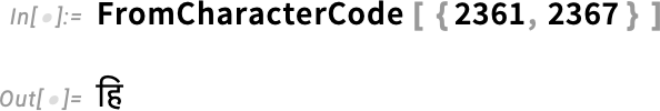
The first character here can stand on its own:

But the second one is basically a modifier that extends the first character (in this particular case adding a vowel sound):

But once the composite हि has been formed it acts “textually” just like a single character, in the sense that, for example, the cursor moves through it in one step. When it appears “computationally” in a string, however, it can still be broken into its constituent Unicode elements:

This kind of setup can be used not only for a language like Hindi but also for European languages that have diacritical marks like umlauts:

Even though this looks like one character—and in Version 13.1 it’s treated like that for “textual” purposes, for example in notebooks—it is ultimately made up of two distinct “Unicode characters”:

In this particular case, though, this can be “normalized” to a single character:

It looks the same, but now it really is just one character:

Here’s a “combined character” that you can form

but for which there’s no single character to which it normalizes:

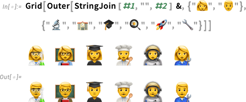
The concept of composite characters applies not only to ordinary text, but also to emojis. For example, take the emoji for a woman

together with the emoji for a microscope

and combine them with the “zero-width-joiner” character (which, needless to say, doesn’t display as anything)

and you get (yes, somewhat bizarrely) a woman scientist!

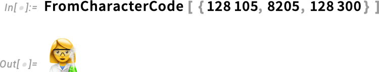
Needless to say, you can do this computationally—though the “calculus” of what’s been defined so far in Unicode is fairly bizarre:

I’m sort of hoping that the future of semantics doesn’t end up being defined by the way emojis combine 😎.

As one last—arguably hacky—example of combining characters, Unicode defines various “two-letter” combinations to be flags. Type then , and you get 🇺🇸!

Once again, this can be made computational:

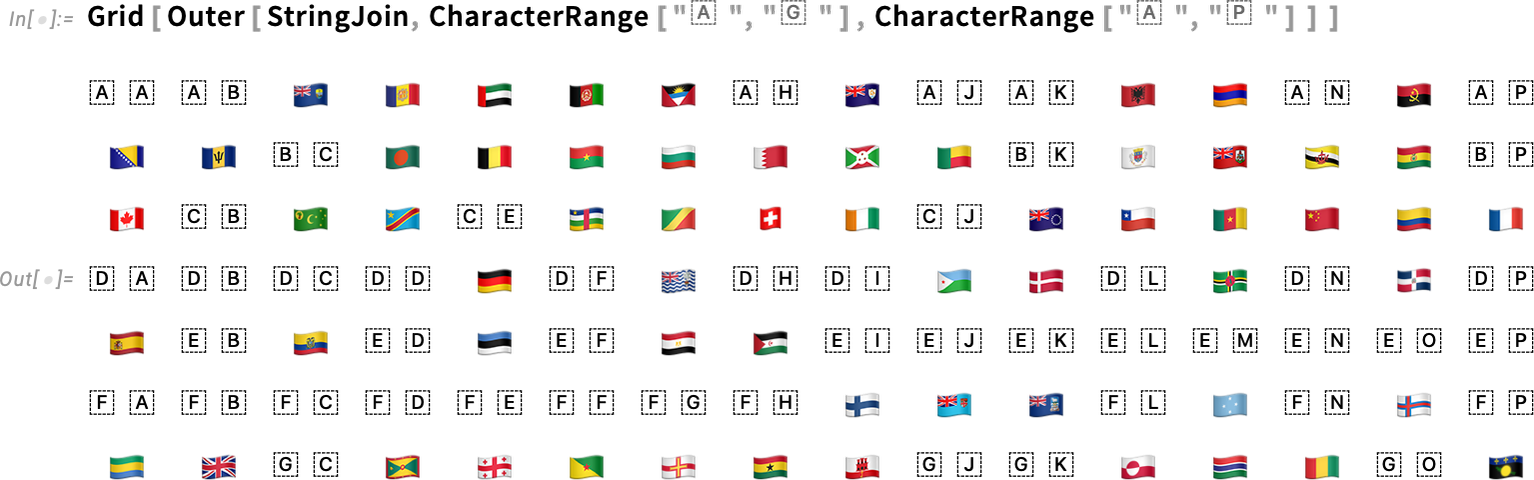
(And, yes, it’s an interesting question what renders here, and what doesn’t. In some operating systems, no flags are rendered, and we have to pull in a special font to do it.)

A Toolbar for Every Notebook (June 2022)

It used to be that the only “special key sequence” one absolutely should know in order to use Wolfram Notebooks was shiftenter. But gradually there have started to be more and more high-profile operations that are conveniently done by “pressing a button”. And rather than expecting people to remember all those special key sequences (or think to look in menus for them) we’ve decided to introduce a toolbar that will be displayed by default in every standard notebook. Version 13.1 has the first iteration of this toolbar. Subsequent versions will support an increasing range of capabilities.

It’s not been easy to design the default toolbar (and we hope you’ll like what we came up with!) The main problem is that Wolfram Notebooks are very general, and there are a great many things you can do with them—which it’s challenging to organize into a manageable toolbar. (Some special types of notebooks have had their own specialized toolbars for a while, which were easier to design by virtue of their specialization.)

So what’s in the toolbar? On the left are a couple of evaluation controls:

means “Evaluate”, and is simply equivalent to pressing shiftret (as its tooltip says). means “Abort”, and will stop a computation. To the right of is the menu shown above. The first part of the menu allows you to choose what will be evaluated. (Don’t forget the extremely useful “Evaluate In Place” that lets you evaluate whatever code you have selected—say to turn RGBColor[1,0,0] in your input into .) The bottom part of the menu gives a couple of more detailed (but highly useful) evaluation controls.

Moving along the toolbar, we next have:

If your cursor isn’t already in a cell, the pulldown allows you to select what type of cell you want to insert (it’s similar to the “tongue” that appears within the notebook). (If your cursor is already inside a cell, then like in a typical word processor, the pulldown will tell you the style that’s being used, and let you reset it.)

gives you a little panel to control to appearance of cells, changing their background colors, frames, dingbats, etc.

Next come cell-related buttons: . The first is for cell structure and grouping:

copies input from above (cmdL). It’s an operation that I, for one, end up doing all the time. I’ll have an input that I evaluate. Then I’ll want to make a modified version of the input to evaluate again, while keeping the original. So I’ll copy the input from above, edit the copy, and evaluate it again.

copies output from above. I don’t find this quite as useful as copy input from above, but it can be helpful if you want to edit output for subsequent input, while leaving the “actual output” unchanged.

The block is all about content in cells. (which you’ll often press repeatedly) is for extending a selection—in effect going ever upwards in an expression tree. (You can get the same effect by pressing ctrl. or by multiclicking, but it’s a lot more convenient to repeatedly press a single button than to have to precisely time your multiclicks.)

is the single-button way to get ctrl= for entering natural language input:

iconizes your selection:

Iconization is something we introduced in Version 11.3, and it’s something that’s proved incredibly useful, particularly for making code easy to read (say by iconizing details of options). (You can also iconize a selection from the right-click menu, or with ctrlcmd'.)

is most relevant for code, and toggles commenting (with ) a selection. brings up a palette for math typesetting. lets you enter that will be converted to Wolfram Language math typesetting. brings up a drawing canvas. inserts a hyperlink (cmdshiftH).

If you’re in a text cell, the toolbar will look different, now sporting a text formatting control:

Most of this is fairly standard. lets you insert “code voice” material. and are still in the toolbar for inserting math into a text cell.

On the right-hand end of the toolbar are three more buttons: . gives you a dialog to publish your notebook to the cloud. opens documentation, either specifically looking up whatever you have selected in the notebook, or opening the front page (“root guide page”) of the main Wolfram Language documentation. Finally, lets you search in your current notebook.

As I mentioned above, what’s in Version 13.1 is just the first iteration of our default toolbar. Expect more features in later versions. One thing that’s notable about the toolbar in general is that it’s 100% implemented in Wolfram Language. And in addition to adding a great deal of flexibility, this also means that the toolbar immediately works on all platforms. (By the way, if you don’t want the toolbar in a particular notebook—or for all your notebooks—just right-click the background of the toolbar to pick that option.)

Polishing the User Interface (June 2022)

We first introduced Wolfram Notebooks with Version 1.0 of Mathematica, in 1988. And ever since then, we’ve been progressively polishing the notebook interface, doing more with every new version.

The ctrl= mechanism for entering natural language (“Wolfram|Alpha-style”) input debuted in Version 10.0—and in Version 13.1 it’s now accessible from the button in the new default notebook toolbar. But what actually is when it’s in a notebook? In the past, it’s been a fairly complex symbolic structure mainly suitable for evaluation. But in Version 13.1 we’ve made it much simpler. And while that doesn’t have any direct effect if you’re just using purely in a notebook, it does have an effect if you copy into another application, like pure-text email. In the past this produced something that would work if pasted back into a notebook, but definitely wasn’t particularly readable. In Version 13.1, it’s now simply the Wolfram Language interpretation of your natural language input:

&#10005

What happens if the computation you do in a notebook generates a huge output? Ever since Version 6.0 we’ve had some form of “output limiter”, but in Version 13.1 it’s become much sleeker and more useful. Here’s a typical example:

&#10005

Talking of big outputs (as well as other things that keep the notebook interface busy), another change in Version 13.1 is the new asynchronous progress overlay on macOS. This doesn’t affect other platforms where this problem had already been solved, but on the Mac changes in the OS had led to a situation where the notebook front end could mysteriously pop to the front on your desktop—a situation that has now been resolved.

One of the slightly unusual user interface features that’s existed ever since Version 1.0 is the Why the Beep? menu item—that lets you get an explanation of any “error beep” that occurs while you’re running the system. The function Beep lets you generate your own beep. And now in Version 13.1 you can use Beep["string"] to set up an explanation of “your beep”, that users can retrieve through the Why the Beep? menu item.

The basic notebook user interface works as much as possible with standard interface elements on all platforms, so that when these elements are updated, we always automatically get the “most modern” look. But there are parts of the notebook interface that are quite special to Wolfram Notebooks and are always custom designed. One that hadn’t been updated for a while is the Preferences dialog—which now in Version 13.1 gets a full makeover:

&#10005

When you tell the Wolfram Language to do something, it normally just goes off and does it, without asking you anything (well, unless it explicitly needs input, needs a password, etc.) But what if there’s something that it might be a good idea to do, though it’s not strictly necessary? What should the user interface for this be? It’s tricky, but I think we now have a good solution that we’ve started deploying in Version 13.1.

In particular, in Version 13.1, there’s an example related to the Wolfram Function Repository. Say you use a function for which an update is available. What now happens is that a blue box is generated that tells you about the update—though it still keeps going with the computation, ignoring the update:

&#10005

If you click the Update Now button in the blue box you can do the update. And then the point is that you can run the computation again (for example, just by pressing shiftenter), and now it’ll use the update. In a sense the core idea is to have an interface where there are potentially multiple passes, and where a computation always runs to completion, but you have an easy way to change how it’s set up, and then run it again.

Scribbling on Notebooks (June 2022)

In Version 12.2 we introduced Canvas as a convenient interface for interactive drawing in notebooks. In Version 13.1 we’re introducing the notion of toggling a canvas on top of any cell.

Given a cell, just select it and press , and you’ll get a canvas:

&#10005

Now you can use the drawing tools in the canvas to create an annotation overlay:

&#10005

If you evaluate the cell, the overlay will stay. (You can get rid of the “canvas wrapper” by applying Normal.)

Graphics, Image, Graph, …? Tell It from the Frame Color (December 2022)

Everything in the Wolfram Language is a symbolic expression. But different symbolic expressions are displayed differently, which is, of course, very useful. So, for example, a graph isn’t displayed in the raw symbolic form

&#10005

but rather as a graph:

&#10005

But let’s say you’ve got a whole collection of visual objects in a notebook. How can you tell what they “really are”? Well, you can click them, and then see what color their borders are. It’s subtle, but I’ve found one quickly gets used to noticing at least the kinds of objects one commonly uses. And in Version 13.2 we’ve made some additional distinctions, notably between images and graphics.

So, yes, the object above is a Graph—and you can tell that because it has a purple border when you click it:

&#10005

This is a Graphics object, which you can tell because it’s got an orange border:

&#10005

And here, now, is an Image object, with a light blue border:

&#10005

For some things, color hints just don’t work, because people can’t remember which color means what. But for some reason, adding color borders to visual objects seems to work very well; it provides the right level of hinting, and the fact that one often sees the color when it’s obvious what the object is helps cement a memory of the color.

In case you’re wondering, there are some others already in use for borders—and more to come. Trees are green (though, yes, ours by default grow down). Meshes are brown:

&#10005

User Interface Conveniences (December 2022)

We first introduced the notebook interface in Version 1 back in 1988. And already in that version we had many of the current features of notebooks—like cells and cell groups, cell styles, etc. But over the past 34 years we’ve been continuing to tweak and polish the notebook interface to make it ever smoother to use.

In Version 13.2 we have some minor but convenient additions. We’ve had the Divide Cell menu item (cmdshiftD) for more than 30 years. And the way it’s always worked is that you click where you want a cell to be divided. Meanwhile, we’ve always had the ability to put multiple Wolfram Language inputs into a single cell. And while sometimes it’s convenient to type code that way, or import it from elsewhere like that, it makes better use of all our notebook and cell capabilities if each independent input is in its own cell. And now in Version 13.2 Divide Cell can make it like that, analyzing multiline inputs to divide them between complete inputs that occur on different lines:

&#10005

Similarly, if you’re dealing with text instead of code, Divide Cell will now divide at explicit line breaks—that might correspond to paragraphs.

In a completely different area, Version 13.1 added a new default toolbar for notebooks, and in Version 13.2 we’re beginning the process of steadily adding features to this toolbar. The main obvious feature that’s been added is a new interactive tool for changing frames in cells. It’s part of the Cell Appearance item in the toolbar:

&#10005

Just click a side of the frame style widget and you’ll get a tool to edit that frame style—and you’ll immediately see any changes reflected in the notebook:

&#10005

If you want to edit all the sides, you can lock the settings together with:

&#10005

Cell frames have always been a useful mechanism for delineating, highlighting or otherwise annotating cells in notebooks. But in the past it’s been comparatively difficult to customize them beyond what’s in the stylesheet you’re using. With the new toolbar feature in Version 13.2 we’ve made it very easy to work with cell frames, making it realistic for custom cell frames to become a routine part of notebook content.

The Elegant Code Project (June 2023)

One of the central goals—and achievements—of the Wolfram Language is to create a computational language that can be used not only as a way to tell computers what to do, but also as a way to communicate computational ideas for human consumption. In other words, Wolfram Language is intended not only to be written by humans (for consumption by computers), but also to be read by humans.

Crucial to this is the broad consistency of the Wolfram Language, as well as its use of carefully chosen natural-language-based names for functions, etc. But what can we do to make Wolfram Language as easy and pleasant as possible to read? In the past we’ve balanced our optimization of the appearance of Wolfram Language between reading and writing. But in Version 13.3 we’ve got the beginnings of our Elegant Code project—to find ways to render Wolfram Language to be specifically optimized for reading.

As an example, here’s a small piece of code (from my An Elementary Introduction to the Wolfram Language), shown in the default way it’s rendered in notebooks:

But in Version 13.3 you can use Format > Screen Environment > Elegant to set a notebook to use the current version of “elegant code”:

(And, yes, this is what we’re actually using for code in this post, as well as some other recent ones.) So what’s the difference? First of all, we’re using a proportionally spaced font that makes the names (here of symbols) easy to “read like words”. And second, we’re adding space between these “words”, and graying back “structural elements” like … and … . When you write a piece of code, things like these structural elements need to stand out enough for you to “see they’re right”. But when you’re reading code, you don’t need to pay as much attention to them. Because the Wolfram Language is so based on “word-like” names, you can typically “understand what it’s saying” just by “reading these words”.

Of course, making code “elegant” is not just a question of formatting; it’s also a question of what’s actually in the code. And, yes, as with writing text, it takes effort to craft code that “expresses itself elegantly”. But the good news is that the Wolfram Language—through its uniquely broad and high-level character—makes it surprisingly straightforward to create code that expresses itself extremely elegantly.

But the point now is to make that code not only elegant in content, but also elegant in formatting. In technical documents it’s common to see math that’s at least formatted elegantly. But when one sees code, more often than not, it looks like something only a machine could appreciate. Of course, if the code is in a traditional programming language, it’ll usually be long and not really intended for human consumption. But what if it’s elegantly crafted Wolfram Language code? Well then we’d like it to look as attractive as text and math. And that’s the point of our Elegant Code project.

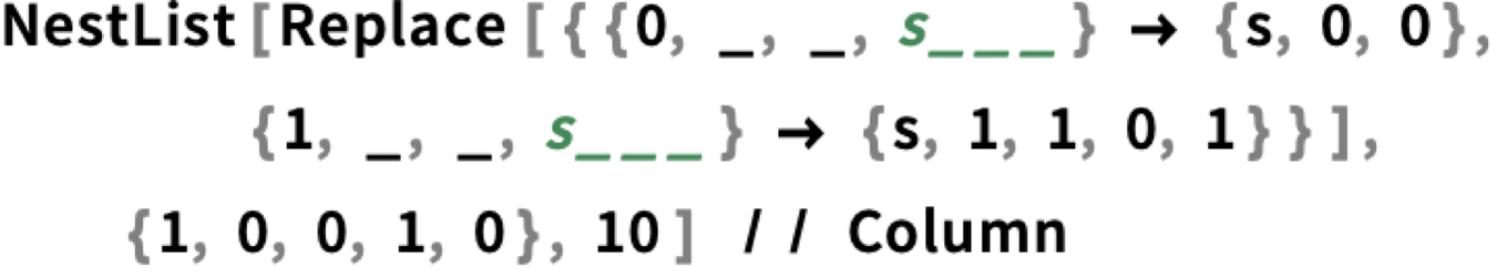
There are many tradeoffs, and many issues to be navigated. But in Version 13.3 we’re definitely making progress. Here’s an example that doesn’t have so many “words”, but where the elegant code formatting still makes the “blocking” of the code more obvious:

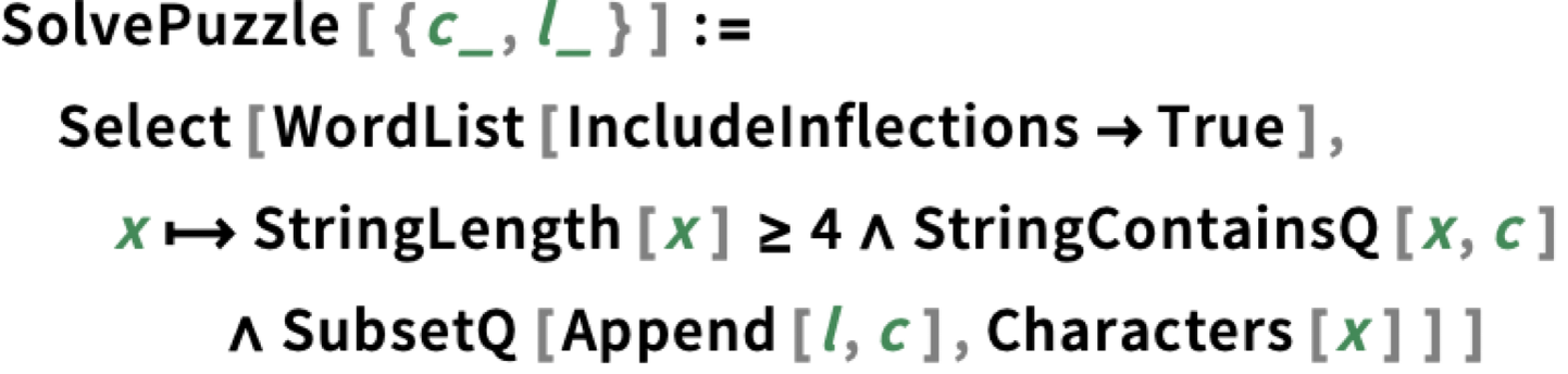
Here’s a slightly longer piece of code, where again the elegant code formatting helps pull out “readable” words, as well as making the overall structure of the code more obvious:

Particularly in recent years, we’ve added many mechanisms to let one write Wolfram Language that’s easier to read. There are the auto operator renderings, like m[[i]] turning into . And then there are things like the notation for pure functions. One particularly important element is Iconize, which lets you show any piece of Wolfram Language input in a visually “iconized” form—which nevertheless evaluates just like the corresponding underlying expression:

Iconize lets you effectively hide details (like large amounts of data, option settings, etc.) But sometimes you want to highlight things. You can do it with Style, Framed, Highlighted—and in Version 13.3, Squiggled:

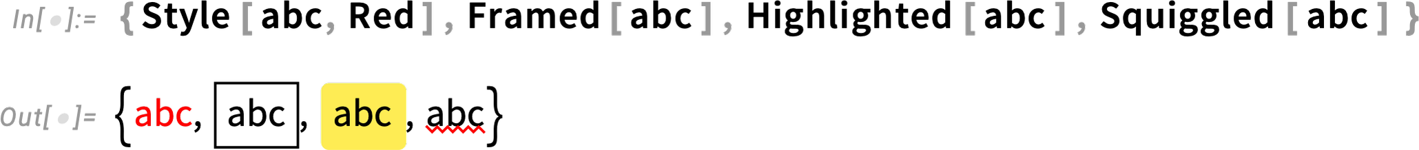
By default, all these constructs persist through evaluation. But in Version 13.3 all of them now have the option StripOnInput, and with this set, you have something that shows up highlighted in an input cell, but where the highlighting is stripped when the expression is actually fed to the Wolfram Language kernel.

These show their highlighting in the notebook:

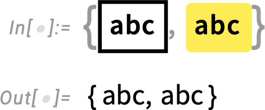
But when used in input, the highlighting is stripped:

For Serious Developers

For Serious Developers (January 2024)

A single line (or less) of Wolfram Language code can do a lot. But one of the remarkable things about the language is that it’s fundamentally scalable: good both for very short programs and very long programs. And since Version 13 there’ve been several advances in handling very long programs. One of them concerns “code editing”.

Standard Wolfram Notebooks work very well for exploratory, expository and many other forms of work. And it’s certainly possible to write large amounts of code in standard notebooks (and, for example, I personally do it). But when one’s doing “software-engineering-style work” it’s both more convenient and more familiar to use what amounts to a pure code editor, largely separate from code execution and exposition. And this is why we have the “package editor”, accessible from File > New > Package/Script. You’re still operating in the notebook environment, with all its sophisticated capabilities. But things have been “skinned” to provide a much more textual “code experience”—both in terms of editing, and in terms of what actually gets saved in .wl files.

Here’s typical example of the package editor in action (in this case applied to our GitLink package):

Several things are immediately evident. First, it’s very line oriented. Lines (of code) are numbered, and don’t break except at explicit newlines. There are headings just like in ordinary notebooks, but when the file is saved, they’re stored as comments with a certain stylized structure:

It’s still perfectly possible to run code in the package editor, but the output won’t get saved in the .wl file:

One thing that’s changed since Version 13 is that the toolbar is much enhanced. And for example there’s now “smart search” that is aware of code structure:

You can also ask to go to a line number—and you’ll immediately see whatever lines of code are nearby:

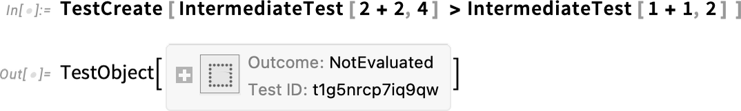
In addition to code editing, another set of features new since Version 13 of importance to serious developers concern automated testing. The main advance is the introduction of a fully symbolic testing framework, in which individual tests are represented as symbolic objects

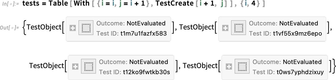
and can be manipulated in symbolic form, then run using functions like TestEvaluate and TestReport:

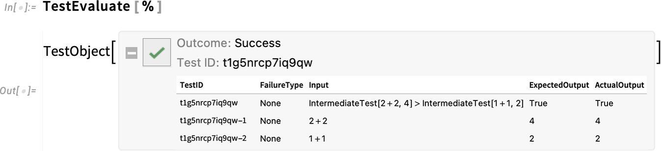
In Version 14.0 there’s another new testing function—IntermediateTest—that lets you insert what amount to checkpoints inside larger tests:

Evaluating this test, we see that the intermediate tests were also run:

Large-Scale Code Editing (June 2022)

One of the great things about the Wolfram Language is that it works well for programs of any scale—from less than a line long to millions of lines long. And for the past several years we’ve been working on expanding our support for very large Wolfram Language programs. Using LSP (Language Server Protocol) we’ve provided the capability for most standard external IDEs to automatically do syntax coloring and other customizations for the Wolfram Language.

In Version 13.1 we’re also adding a couple of features that make large-scale code editing in notebooks more convenient. The first—and widely requested—is block indent and outdent of code. Select the lines you want to indent or outdent and simply press tab or shifttab to indent or outdent them:

&#10005

Ever since Version 6.0 we’ve had the ability to work with .wl package files (as well as .wls script files) using our notebook editing system. A new default feature in Version 13.1 is numbering of all code lines that appear in the underlying file (and, yes, we correctly align line numbers accounting for the presence of non-code cells):

&#10005

So now, for example, if you get a syntax error from Get or a related function, you’ll immediately be able to use the line number it reports to find where it occurs in the underlying file.

Create Your Own “Guide to Functions” Pages (June 2022)

An important part of the built-in documentation for the Wolfram Language are what we call “guide pages”—pages like the following that organize functions (and other constructs) to give an overall “cognitive map” and summary of some area:

&#10005

In Version 13.1 it’s now easy to create your own custom guide pages. You can list built-in functions or other constructs, as well as things from the Wolfram Function Repository and other repositories.

Go to the “root page” of the Documentation Center and press the icon:

&#10005

You’ll get a blank custom guide page:

&#10005

Fill in the guide page however you want, then use Deploy to deploy the page either locally, or to your cloud account. Either way, the page will now show up in the menu from the top of the root guide page (and they’ll also show up in search):

&#10005

You might end up creating just one custom guide page for your favorite functions. Or you might create several, say one for each task or topic you commonly deal with. Guide pages aren’t about putting in the effort to create full-scale documentation; they’re much more lightweight, and aimed more at providing quick (“what was that function called?”) reminders and “big-picture” maps—leveraging all the specific function and other documentation that already exists.

Brighter, Better Syntax Coloring (December 2022)

How do we make it as easy as possible to type correct Wolfram Language code? This is a question we’ve been working on for years, gradually inventing more and more mechanisms and solutions. In Version 13.2 we’ve made some small tweaks to a mechanism that’s actually been in the system for many years, but the changes we’ve made have a substantial effect on the experience of typing code.

One of the big challenges is that code is typed “linearly”—essentially (apart from 2D constructs) from left to right. But (just like in natural languages like English) the meaning is defined by a more hierarchical tree structure. And one of the issues is to know how something you typed fits into the tree structure.

Something like this is visually obvious quite locally in the “linear” code you typed. But sometimes what defines the tree structure is quite far away. For example, you might have a function with several arguments that are each large expressions. And when you’re looking at one of the arguments it may not be obvious what the overall function is. And part of what we’re now emphasizing more strongly in Version 13.2 is dynamic highlighting that shows you “what function you’re in”.

It’s highlighting that appears when you click. So, for example, this is the highlighting you get clicking at several different positions in a simple expression:

Here’s an example “from the wild” showing you that if you type at the position of the cursor, you’ll be adding an argument to the ContourPlot function:

&#10005

But now let’s click in a different place:

&#10005

Here’s a smaller example:

&#10005

Notice that we’re highlighting both the enclosing grouping {…} and the enclosing function head.

We’ve had the basic capability for this kind of highlighting for nearly a decade. But in Version 13.2 we’re making it much bolder, and we’ve subtly tweaked what highlighting shows up when. This may seem like a detail, but I, for example, have found it quite transformative in the way that I actually type code.

In the past I often found myself multiclicking to figure out the structure of the code. But now I just have to click and the highlighting is bright enough to be immediately obvious, even if it’s quite far away in the linear rendering of the code.

It’s also important that the highlighting colors for function heads and for grouping constructs are now much more distinct. In the past, they were both shades of green, which were hard to distinguish and understand. With the Version 13.2 colors one quickly gets used to how things are set up, and it’s easy to get a sense of the structure of an expression. And having these two colors (as opposed to more, or fewer) seems to be about right in terms of giving information, but not giving so much that it’s hard to assimilate.

Even Easier to Type: Affordances for Wolfram Language Input (June 2023)

Back in 1988 when what’s now Wolfram Language first existed, the only way to type it was like ordinary text. But gradually we’ve introduced more and more “affordances” to make it easier and faster to type correct Wolfram Language input. In 1996, with Version 3, we introduced automatic spacing (and spanning) for operators, as well as brackets that flashed when they matched—and things like -> being automatically replaced by . Then in 2007, with Version 6, we introduced—with some trepidation at first—syntax coloring. We’d had a way to request autocompletion of a symbol name all the way back to the beginning, but it’d never been good or efficient enough for us to make it happen all the time as you type. But in 2012, for Version 9, we created a much more elaborate autocomplete system—that was useful and efficient enough that we turned it on for all notebook input. A key feature of this autocomplete system was its context-sensitive knowledge of the Wolfram Language, and how and where different symbols and strings typically appear. Over the past decade, we’ve gradually refined this system to the point where I, for one, deeply rely on it.

In recent versions, we’ve made other “typability” improvements. For example, in Version 12.3, we generalized the -> to transformation to a whole collection of “auto operator renderings”. Then in Version 13.0 we introduced “automatching” of brackets, in which, for example, if you enter [ at the end of what you’re typing, you’ll automatically get a matching ].

Making “typing affordances” work smoothly is a painstaking and tricky business. But in every recent version we’ve steadily been adding more features that—in very “natural” ways—make it easier and faster to type Wolfram Language input.

In Version 13.3 one major change is an enhancement to autocompletion. Instead of just showing pure completions in which characters are appended to what’s already been typed, the autocompletion menu now includes “fuzzy completions” that fill in intermediate characters, change capitalization, etc.

So, for example, if you type “lp” you now get ListPlot as a completion (the little underlines indicate where the letters you actually type appear):

From a design point of view one thing that’s important about this is that it further removes the “short name” premium—and weights things even further on the side of wanting names that explain themselves when they’re read, rather than that are easy to type in an unassisted way. With the Wolfram Function Repository it’s become increasingly common to want to type ResourceFunction. And we’d been thinking that perhaps we should have a special, short notation for that. But with the new autocompletion, one can operationally just press three keys—rfenter—to get to ResourceFunction:

When one designs something and gets the design right, people usually don’t notice; things just “work as they expect”. But when there’s a design error, that’s when people notice—and are frustrated by—the design. But then there’s another case: a situation where, for example, there are two things that could happen, and sometimes one wants one, and sometimes the other. In doing the design, one has to pick a particular branch. And when this happens to be the branch people want, they don’t notice, and they’re happy. But if they want the other branch, it can be confusing and frustrating.

In the design of the Wolfram Language one of the things that has to be chosen is the precedence for every operator: a + b × c means a + (b × c) because × has higher precedence than +. Often the correct order of precedences is fairly obvious. But sometimes it’s simply impossible to make everyone happy all the time. And so it is with and &. It’s very convenient to be able to add & at the end of something you type, and make it into a pure function. But that means if you type a b & it’ll turn the whole thing into a function: a b &. When functions have options, however, one often wants things like name function. The natural tendency is to type this as name body &. But this will mean (name body) & rather than name (body &). And, yes, when you try to run the function, it’ll notice it doesn’t have correct arguments and options specified. But you’d like to know that what you’re typing isn’t right as soon as you type it. And now in Version 13.3 we have a mechanism for that. As soon as you enter & to “end a function”, you’ll see the extent of the function flash:

And, yup, you can see that’s wrong. Which gives you the chance to fix it as:

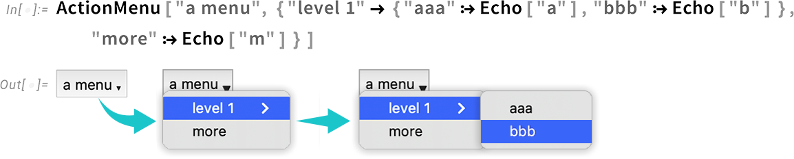
There’s another notebook-related update in Version 13.3 that isn’t directly related to typing, but will help in the construction of easy-to-navigate user interfaces. We’ve had ActionMenu since 2007—but it’s only been able to create one-level menus. In Version 13.3 it’s been extended to arbitrary hierarchical menus:

Again not directly related to typing, but now relevant to managing and editing code, there’s an update in Version 13.3 to package editing in the notebook interface. Bring up a .wl file and it’ll appear as a notebook. But its default toolbar is different from the usual notebook toolbar (and is newly designed in Version 13.3):

Go To now gives you a way to immediately go to the definition of any function whose name matches what you type, as well as any section, etc.:

The numbers on the right here are code line numbers; you can also go directly to a specific line number by typing :nnn.