New in 14: Geometry & Graphs
Two years ago we released Version 13.0 of Wolfram Language. Here are the updates in geometry and graphs since then, including the latest features in 14.0. The contents of this post are compiled from Stephen Wolfram’s Release Announcements for 13.1, 13.2, 13.3 and 14.0.
Geometric Computation
Euclid Redux: The Advance of Synthetic Geometry (January 2024)
One might say it’s been two thousand years in the making. But four years ago (Version 12) we began to introduce a computable version of Euclid-style synthetic geometry.
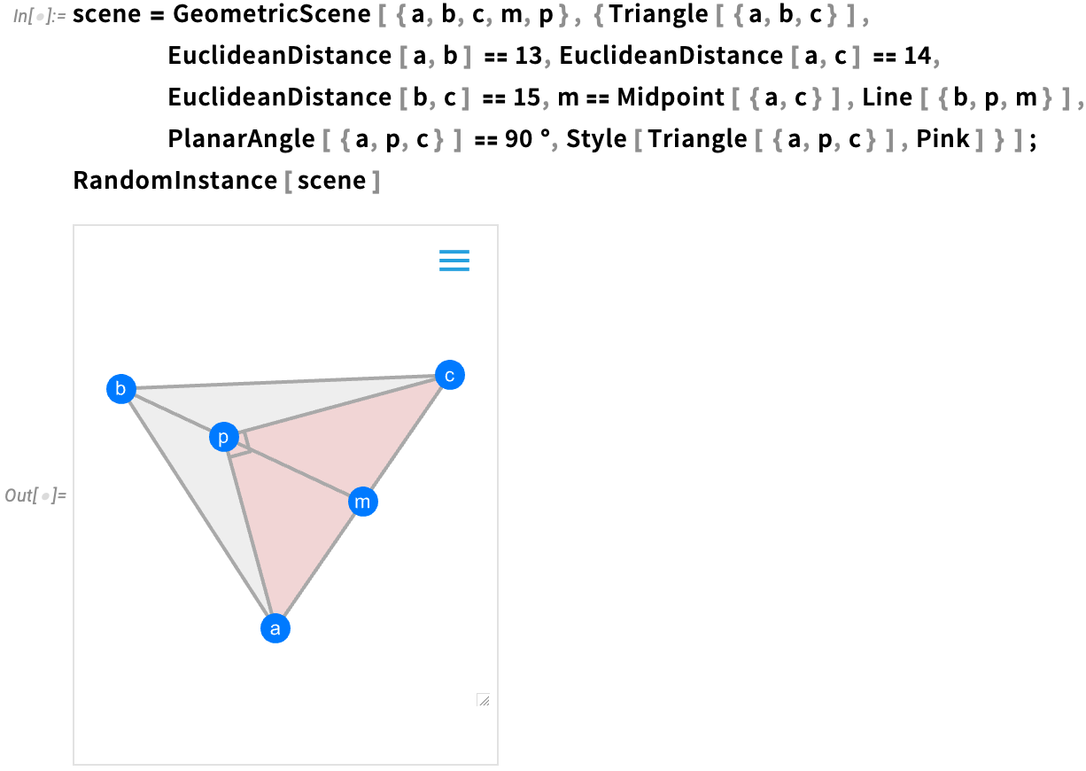
The idea is to specify geometric scenes symbolically by giving a collection of (potentially implicit) constraints:

We can then generate a random instance of geometry consistent with the constraints—and in Version 14 we’ve considerably enhanced our ability to make sure that geometry will be “typical” and non-degenerate:

But now a new feature of Version 14 is that we can find values of geometric quantities that are determined by the constraints:

Here’s a slightly more complicated case:

And here we’re now solving for the areas of two triangles in the figure:

We’ve always been able to give explicit styles for particular elements of a scene:
Now one of the new features in Version 14 is being able to give general “geometric styling rules”, here just assigning random colors to each element:

3D Voronoi! (June 2022)
There are some capabilities that—over the course of years—have been requested over and over again. In the past these have included infinite undo, high dpi displays, multiple axis plots, and others. And I’m happy to say that most of these have now been taken care of. But there’s one—seemingly obscure—“straggler” that I’ve heard about for well over 25 years, and that I’ve actually also wanted myself quite a few times: 3D Voronoi diagrams. Well, in Version 13.1, they’re here.
Set up 25 random points in 3D:

Now make a Voronoi mesh for these points:

To “see inside” we can use opacity:

Why was this so hard? In a Voronoi there’s a cell that surrounds each original point, and includes everywhere that’s closer to that point than to any other. We’ve had 2D Voronoi meshes for a long time:

But there’s something easier about the 2D case. The issue is not so much the algorithm for generating the cells as it is how the cells can be represented in such a way that they’re useful for subsequent computations. In the 2D case each cell is just a polygon.
But in the 3D case the cells are polyhedra, and to make a Voronoi mesh we have to have a polyhedral mesh where all the polyhedra fit together. And it’s taken us many years to build the large tower of computational geometry necessary to support this. There’s a somewhat simpler case based purely on cells that are always either simplices or hexahedra—that we’ve used for finite-element solutions to PDEs for a while. But in a true 3D Voronoi that’s not enough: the cells can be any (convex) polyhedral shape.
Here are the “puzzle piece” cells for the 3D Voronoi mesh we made above:

Reconstructing Geometry from Point Clouds (June 2022)
Pick 500 random points inside an annulus:

Version 13.1 now has a general function reconstructing geometry from a cloud of points:

(Of course, given only a finite number of points, the reconstruction can’t be expected to be perfect.)
The function also works in 3D:


ReconstructionMesh is a general superfunction that uses a variety of methods, including extended versions of the functions ConcaveHullMesh and GradientFittedMesh that were introduced in Version 13.0. And in addition to reconstructing “solid objects”, it can also reconstruct lower-dimensional things like curves and surfaces:

A related function new in Version 13.1 is EstimatedPointNormals, which reconstructs not the geometry itself, but normal vectors to each element in the geometry:

More, Stronger Computational Geometry (June 2023)
We originally introduced computational geometry in a serious way into the Wolfram Language a decade ago. And ever since then we’ve been building more and more capabilities in computational geometry.
We’ve had RegionDistance for computing the distance from a point to a region for a decade. In Version 13.3 we’ve now extended RegionDistance so it can also compute the shortest distance between two regions:
We’ve also introduced RegionFarthestDistance which computes the furthest distance between any two points in two given regions:
Another new function in Version 13.3 is RegionHausdorffDistance which computes the largest of all shortest distances between points in two regions; in this case it gives a closed form:

Another pair of new functions in Version 13.3 are InscribedBall and CircumscribedBall—which give (n-dimensional) spheres that, respectively, just fit inside and outside regions you give:

In the past several versions, we’ve added functionality that combines geo computation with computational geometry. Version 13.3 has the beginning of another initiative—introducing abstract spherical geometry:
This works for spheres in any number of dimensions:

In addition to adding functionality, Version 13.3 also brings significant speed enhancements (often 10x or more) to some core operations in 2D computational geometry—making things like computing this fast even though it involves complicated regions:

Publishing to Augmented + Virtual Reality (June 2023)
Throughout the history of the Wolfram Language 3D visualization has been an important capability. And we’re always looking for ways to share and communicate 3D geometry. Already back in the early 1990s we had experimental implementations of VR. But at the time there wasn’t anything like the kind of infrastructure for VR that would be needed to make this broadly useful. In the mid-2010s we then introduced VR functionality based on Unity—that provides powerful capabilities within the Unity ecosystem, but is not accessible outside.
Today, however, it seems there are finally broad standards emerging for AR and VR. And so in Version 13.3 we’re able to begin delivering what we hope will provide widely accessible AR and VR deployment from the Wolfram Language.
At a underlying level what we’re doing is to support the USD and GLTF geometry representation formats. But we’re also building a higher-level interface that allows anyone to “publish” 3D geometry for AR and VR.
Given a piece of geometry (which for now can’t involve too many polygons), all you do is apply ARPublish:

The result is a cloud object that has a certain underlying UUID, but is displayed in a notebook as a QR code. Now all you do is look at this QR code with your phone (or tablet, etc.) camera, and press the URL it extracts.
The result will be that the geometry you published with ARPublish now appears in AR on your phone:

Move your phone and you’ll see that your geometry has been realistically placed into the scene. You can also go to a VR “object” mode in which you can manipulate the geometry on your phone.
“Under the hood” there are some slightly elaborate things going on—particularly in providing the appropriate data to different kinds of phones. But the result is a first step in the process of easily being able to get AR and VR output from the Wolfram Language—deployed in whatever devices support AR and VR.
Graphs
The Tree Story Continues (January 2024)
Trees are useful. We first introduced them as basic objects in the Wolfram Language only in Version 12.3. But now that they’re there, we’re discovering more and more places they can be used. And to support that, we’ve been adding more and more capabilities to them.
One area that’s advanced significantly since Version 13 is the rendering of trees. We tightened up the general graphic design, but, more importantly, we introduced many new options for how rendering should be done.
For example, here’s a random tree where we’ve specified that for all nodes only 3 children should be explicitly displayed: the others are elided away:

Here we’re adding several options to define the rendering of the tree:

By default, the branches in trees are labeled with integers, just like parts in an expression. But in Version 13.1 we added support for named branches defined by associations:

Our original conception of trees was very centered around having elements one would explicitly address, and that could have “payloads” attached. But what became clear is that there were applications where all that mattered was the structure of the tree, not anything about its elements. So we added UnlabeledTree to create “pure trees”:

Trees are useful because many kinds of structures are basically trees. And since Version 13 we’ve added capabilities for converting trees to and from various kinds of structures. For example, here’s a simple Dataset object:

You can use ExpressionTree to convert this to a tree:

And TreeExpression to convert it back:

We’ve also added capabilities for converting to and from JSON and XML, as well as for representing file directory structures as trees:

Trees Continue to Grow 🌱🌳 (June 2022)
In Version 12.3 we introduced Tree as a new fundamental construct in the Wolfram Language. In Version 13.0 we added a variety of styling options for trees, and in Version 13.1 we’re adding more styling as well as a variety of new fundamental features.
An important update to the fundamental Tree construct in Version 13.1 is the ability to name branches at each node, by giving them in an association:

All tree functions now include support for associations:

In many uses of trees the labels of nodes are crucial. But particularly in more abstract applications one often wants to deal with unlabeled trees. In Version 13.1 the function UnlabeledTree (roughly analogously to UndirectedGraph) takes a labeled tree, and basically removes all visible labels. Here is a standard labeled tree

and here’s the unlabeled analog:

In Version 12.3 we introduced ExpressionTree for deriving trees from general symbolic expressions. Our plan is to have a wide range of “special trees” appropriate for representing different specific kinds of symbolic expressions. We’re beginning this process in Version 13.1 by, for example, having the concept of “Dataset trees”. Here’s ExpressionTree converting a dataset to a tree:

And now here’s TreeExpression “inverting” that, and producing a dataset:

(Remember the convention that *Tree functions return a tree; while Tree* functions take a tree and return something else.)
Here’s a “graph rendering” of a more complicated dataset tree:

The new function TreeLeafCount lets you count the total number of leaf nodes on a tree (basically the analog of LeafCount for a general symbolic expression):
Another new function in Version 13.1 that’s often useful in getting a sense of the structure of a tree without inspecting every node is RootTree. Here’s a random tree:

RootTree can get a subtree that’s “close to the root”:

It can also get a subtree that’s “far from the leaves”, in this case going down to elements that are at level –2 in the tree:

In some ways the styling of trees is like the styling of graphs—though there are some significant differences as a result of the hierarchical nature of trees. By default, options inserted into a particular tree element affect only that tree element:

But you can give rules that specify how elements in the subtree below that element are affected:

In Version 13.1 there is now detailed control available for styling both nodes and edges in the tree. Here’s an example that gives styling for parent edges of nodes:

Options like TreeElementStyle determine styling from the positions of elements. TreeElementStyleFunction, on the other hand, determines styling by applying a function to the data at each node:

This uses both data and position information for each node:

In analogy with VertexShapeFunction for graphs, TreeElementShapeFunction provides a general mechanism to specify how nodes of a tree should be rendered. This named setting for TreeElementShapeFunction makes every node be displayed as a circle:

Displaying Large Trees, and Making More (December 2022)
We first introduced trees as a fundamental structure in Version 12.3, and we’ve been enhancing them ever since. In Version 13.1 we added many options for determining how trees are displayed, but in Version 13.2 we’re adding another, very important one: the ability to elide large subtrees.
Here’s a size-200 random tree with every branch shown:

And here’s the same tree with every node being told to display a maximum of 3 children:

And, actually, tree elision is convenient enough that in Version 13.2 we’re doing it by default for any node that has more than 10 children—and we’ve introduced the global $MaxDisplayedChildren to determine what that default limit should be.
Another new tree feature in Version 13.2 is the ability to create trees from your file system. Here’s a tree that goes down 3 directory levels from my Wolfram Desktop installation directory:


