Two years ago we released Version 13.0 of Wolfram Language. Here are the updates in the core language since then, including the latest features in 14.0. The contents of this post are compiled from Stephen Wolfram’s Release Announcements for 13.1, 13.2, 13.3 and 14.0.

More Core Language

Core Language (January 2024)

What are the primitives from which we can best build our conception of computation? That’s at some level the question I’ve been asking for more than four decades, and what’s determined the functions and structures at the core of the Wolfram Language.

And as the years go by, and we see more and more of what’s possible, we recognize and invent new primitives that will be useful. And, yes, the world—and the ways people interact with computers—change too, opening up new possibilities and bringing new understanding of things. Oh, and this year there are LLMs which can “get the intellectual sense of the world” and suggest new functions that can fit into the framework we’ve created with the Wolfram Language. (And, by the way, there’ve also been lots of great suggestions made by the audiences of our design review livestreams.)

One new construct added in Version 13.1—and that I personally have found very useful—is Threaded. When a function is listable—as Plus is—the top levels of lists get combined:

But sometimes you want one list to be “threaded into” the other at the lowest level, not the highest. And now there’s a way to specify that, using Threaded:

In a sense, Threaded is part of a new wave of symbolic constructs that have “ambient effects” on lists. One very simple example (introduced in 2015) is Nothing:

Another, introduced in 2020, is Splice:

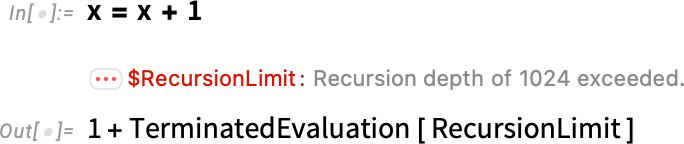
An old chestnut of Wolfram Language design concerns the way infinite evaluation loops are handled. And in Version 13.2 we introduced the symbolic construct TerminatedEvaluation to provide better definition of how out-of-control evaluations have been terminated:

In a curious connection, in the computational representation of physics in our recent Physics Project, the direct analog of nonterminating evaluations are what make possible the seemingly unending universe in which we live.

But what is actually going on “inside an evaluation”, terminating or not? I’ve always wanted a good representation of this. And in fact back in Version 2.0 we introduced Trace for this purpose:

But just how much detail of what the evaluator does should one show? Back in Version 2.0 we introduced the option TraceOriginal that traces every path followed by the evaluator:

But often this is way too much. And in Version 14.0 we’ve introduced the new setting TraceOriginal→Automatic, which doesn’t include in its output evaluations that don’t do anything:

This may seem pedantic, but when one has an expression of any substantial size, it’s a crucial piece of pruning. So, for example, here’s a graphical representation of a simple arithmetic evaluation, with TraceOriginal→True:

And here’s the corresponding “pruned” version, with TraceOriginal→Automatic:

(And, yes, the structures of these graphs are closely related to things like the causal graphs we construct in our Physics Project.)

In the effort to add computational primitives to the Wolfram Language, two new entrants in Version 14.0 are Comap and ComapApply. The function Map takes a function f and “maps it” over a list:

Comap does the “mathematically co-” version of this, taking a list of functions and “comapping” them onto a single argument:

Why is this useful? As an example, one might want to apply three different statistical functions to a single list. And now it’s easy to do that, using Comap:

By the way, as with Map, there’s also an operator form for Comap:

Comap works well when the functions it’s dealing with take just one argument. If one has functions that take multiple arguments, ComapApply is what one typically wants:

Talking of “co-like” functions, a new function added in Version 13.2 is PositionSmallest. Min gives the smallest element in a list; PositionSmallest instead says where the smallest elements are:

One of the important objectives in the Wolfram Language is to have as much as possible “just work”. When we released Version 1.0 strings could be assumed just to contain ordinary ASCII characters, or perhaps to have an external character encoding defined. And, yes, it could be messy not to know “within the string itself” what characters were supposed to be there. And by the time of Version 3.0 in 1996 we’d become contributors to, and early adopters of, Unicode, which provided a standard encoding for “16-bits’-worth” of characters. And for many years this served us well. But in time—and particularly with the growth of emoji—16 bits wasn’t enough to encode all the characters people wanted to use. So a few years ago we began rolling out support for 32-bit Unicode, and in Version 13.1 we integrated it into notebooks—in effect making strings something much richer than before:

And, yes, you can use Unicode everywhere now:

So Much Got Faster, Stronger, Sleeker (January 2024)

With every new version of Wolfram Language we add new capabilities to extend yet further the domain of the language. But we also put a lot of effort into something less immediately visible: making existing capabilities faster, stronger and sleeker.

And in Version 14 two areas where we can see some examples of all these are dates and quantities. We introduced the notion of symbolic dates (DateObject, etc.) nearly a decade ago. And over the years since then we’ve built many things on this structure. And in the process of doing this it’s become clear that there are certain flows and paths that are particularly common and convenient. At the beginning what mattered most was just to make sure that the relevant functionality existed. But over time we’ve been able to see what should be streamlined and optimized, and we’ve steadily been doing that.

In addition, as we’ve worked towards new and different applications, we’ve seen “corners” that need to be filled in. So, for example, astronomy is an area we’ve significantly developed in Version 14, and supporting astronomy has required adding several new “high-precision” time capabilities, such as the TimeSystem option, as well as new astronomy-oriented calendar systems. Another example concerns date arithmetic. What should happen if you want to add a month to January 30? Where should you land? Different kinds of business applications and contracts make different assumptions—and so we added a Method option to functions like DatePlus to handle this. Meanwhile, having realized that date arithmetic is involved in the “inner loop” of certain computations, we optimized it—achieving a more than 100x speedup in Version 14.0.

Wolfram|Alpha has been able to deal with units ever since it was first launched in 2009—now more than 10,000 of them. And in 2012 we introduced Quantity to represent quantities with units in the Wolfram Language. And over the past decade we’ve been steadily smoothing out a whole series of complicated gotchas and issues with units. For example, what does 100°C + 20°C mean? Well, the 20°C isn’t really the same kind of thing as the 100°C. And now in Wolfram Language we have a systematic way to handle this, by distinguishing temperature and temperature difference units—so that we now write 100°C +

At first our priority with Quantity was to get it working as broadly as possible, and to integrate it as widely as possible into computations, visualizations, etc. across the system. But as its capabilities have expanded, so have its uses, repeatedly driving the need to optimize its operation for particular common cases. And indeed between Version 13 and Version 14 we’ve dramatically sped up many things related to Quantity, often by factors of 1000 or more.

Talking of speedups, another example—made possible by new algorithms operating on multithreaded CPUs—concerns polynomials. We’ve worked with polynomials in Wolfram Language since Version 1, but in Version 13.2 there was a dramatic speedup of up to 1000x on operations like polynomial factoring.

In addition, a new algorithm in Version 14.0 dramatically speeds up numerical solutions to polynomial and transcendental equations—and, together with the new MaxRoots options, allows us, for example, to pick off a few roots from a degree-one-million polynomial

or to find roots of a transcendental equation that we could not even attempt before without pre-specifying bounds on their values:

Another “old” piece of functionality with recent enhancement concerns mathematical functions. Ever since Version 1.0 we’ve set up mathematical functions so that they can be computed to arbitrary precision:

But in recent versions we’ve wanted to be “more precise about precision”, and to be able to rigorously compute just what range of outputs are possible given the range of values provided as input:

But every function for which we do this effectively requires a new theorem, and we’ve been steadily increasing the number of functions covered—now more than 130—so that this “just works” when you need to use it in a computation.

The ExprStruct Data Structure (June 2022)

In the Wolfram Language expressions normally have two aspects: they have a structure, and they have a meaning. Thus, for example, Plus[1,1] has both a definite tree structure

&#10005

and has a value:

&#10005

In the normal operation of the Wolfram Language, the evaluator is automatically applied to all expressions, and essentially the only way to avoid evaluation by the evaluator is to insert “wrappers” like Hold and Inactive that necessarily change the structure of expressions.

In Version 13.1, however, there’s a new way to handle “unevaluated” expressions: the "ExprStruct" data structure. ExprStructs represent expressions as raw data structures that are never directly seen by the evaluator, but can nevertheless be structurally manipulated.

This creates an ExprStruct corresponding to the expression {1,2,3,4}:

&#10005

This structurally wraps Total around the list, but does no evaluation:

&#10005

One can also see this by “visualizing” the data structure:

&#10005

Normal takes an ExprStruct object and converts it to a normal expression, to which the evaluator is automatically applied:

&#10005

One can do a variety of essentially structural operations directly on an ExprStruct. This applies Plus, then maps Factorial over the resulting ExprStruct:

&#10005

The result is an ExprStruct representing an unevaluated expression:

&#10005

With "MapImmediateEvaluate" there is an evaluation done each time the mapping operation generates an expression:

&#10005

One powerful use of ExprStruct is in doing code transformations. And in a typical case one might want to import expressions from, say, a .wl file, then manipulate them in ExprStruct form. In Version 13.1 Import now supports an ExprStructs import element:

&#10005

This selects expressions that correspond to definitions, in the sense that they have SetDelayed as their head:

&#10005

Here’s a visualization of the first one:

&#10005

Yet More Language Convenience Functions (June 2022)

In every version of the Wolfram Language we try to add new functions that will make general programs easier to write and easier to read. In Version 13.1 the most important such function is Threaded. But there are quite a few others as well.

First in our collection for Version 13.1 is DeleteElements, which deletes specified elements from a list. It’s like Complement, except that it doesn’t reorder the list (analogous to the way DeleteDuplicates removes duplicate elements, without reordering in the way that Union does):

DeleteElements also allows more detailed control of how many copies of an element can be deleted. Here it is up to 2 b’s and 3 c’s:

Talking of DeleteDuplicates, another new function in Version 13.1 is DeleteAdjacentDuplicates:

We’ve had Union, Intersection and Complement since Version 1.0. In Version 13.1 we’re adding SymmetricDifference: find elements that (in the 2-argument case) are in one list or the other, but not both. For example, what countries are in the G20 or the EU, but not both?

Let’s say you have several lists, and you want to know what elements are unique to just one of these lists, and don’t occur in multiple lists. The new UniqueElements tells one.

As an example, this tells us which letters uniquely occur in various alphabets:

We’ve had Map and Apply, with short forms /@ and @@, ever since Version 1.0. In Version 4.0 we added @@@ to represent Apply[f,expr,1]. But we never added a separate function to correspond to @@@. And over the years, there’ve been quite a few occasions where I’ve basically wanted, for example, to do something like “Fold[@@@, ...]”. Obviously Fold[Apply[#1,#2,1]&,...] would work. But it feels as if there’s a “missing” named function. Well, in Version 13.1, we added it: MapApply is equivalent to @@@:

Another small convenience added in Version 13.1 is SameAs—essentially an operator form of SameQ. Why is such a construct needed? Well, there are always tradeoffs in language design. And back in Version 1.0 we decided to make SameQ work with any number of arguments (so you can test whether a whole sequence of things are the same). But this means that for consistency SameQ[expr] must always return True—so it’s not available as an operator of SameQ. And that’s why now in Version 13.1 we’re adding SameAs, that joins the family of operator-form functions like EqualTo and GreaterThan:

Procedural programming—often with “variables hanging out”—isn’t the preferred style for most Wolfram Language code. But sometimes it’s the most convenient way to do things. And in Version 13.1 we’ve add a small piece of streamlining by introducing the function Until. Ever since Version 1.0 we’ve had While[test,body] which repeatedly evaluates body while test is True. But if test isn’t True even at first, While won’t ever evaluate body. Until[test,body] does things the other way around: it evaluates body until test becomes True. So if test isn’t True at first, Until will still evaluate body once, in effect only looking at the test after it’s evaluated the body.

Last but not least in the list of new core language functions in Version 13.1 is ReplaceAt. Replace attempts to apply a replacement rule to a complete expression—or a whole level in an expression. ReplaceAll (/.) does the same thing for all subparts of an expression. But quite often one wants more control over where replacements are done. And that’s what ReplaceAt provides:

An important feature is that it also has an operator form:

Why is this important? The answer is that it gives a symbolic way to specify not just what replacement is made, but also where it is made. And for example this is what’s needed in specifying steps in proofs, say as generated by FindEquationalProof.

Symbolic Testing Framework 13.3 (June 2023)

The Wolfram Language is by many measures one of the world’s most complex pieces of software engineering. And over the decades we’ve developed a large and powerful system for testing and validating it. A decade ago—in Version 10—we began to make some of our internal tools available for anyone writing Wolfram Language code. Now in Version 13.3 we’re introducing a more streamlined—and “symbolic”—version of our testing framework.

The basic idea is that each test is represented by a symbolic TestObject, created using TestCreate:

On its own, TestObject is an inert object. You can run the test it represents using TestEvaluate:

Each test object has a whole collection of properties, some of which only get filled in when the test is run:

It’s very convenient to have symbolic test objects that one can manipulate using standard Wolfram Language functions, say selecting tests with particular features, or generating new tests from old. And when one builds a test suite, one does it just by making a list of test objects.

This makes a list of test objects (and, yes, there’s some trickiness because TestCreate needs to keep unevaluated the expression that’s going to be tested):

But given these tests, we can now generate a report from running them:

TestReport has various options that allow you to monitor and control the running of a test suite. For example, here we’re saying to echo every "TestEvaluated" event that occurs:

Dates, Times & Units

Yet More Date-Handling Details (June 2023)

We first introduced dates into Wolfram Language in Version 2.0, and we introduced modern date objects in Version 10.0. But to really make dates fully computable, there are many detailed cases to consider. And in Version 13.1 we’re dealing with yet another of them. Let’s say you’ve got the date January 31, 2022. What date is one month later—given that there’s no February 31, 2022?

If we define a month “physically”, it corresponds to a certain fractional number of days:

And, yes, we can use this to decide what is a month after January 31, 2022:

Slightly confusing here is that we’re dealing with date objects of “day” granularity. We can see more if we go down to the level of minutes:

If one’s doing something like astronomy, this kind of “physical” date computation is probably what one wants. But if one’s doing everyday “human” activities, it’s almost certainly not what one wants; instead, one wants to land on some calendar date or another.

Here’s the default in the Wolfram Language:

But now in Version 13.1 we can parametrize more precisely what we want. This default is what we call "RollBackward": wherever we “land” by doing the raw date computation, we “roll backward” to the first valid date. An alternative is "RollForward":

Whatever method one uses, there are going to be weird cases. Let’s say we start with several consecutive dates:

With "RollBackward" we have the weirdness of repeating February 28:

With "RollForward" we have the weirdness of repeating March 1:

Is there any alternative? Yes, we can use "RollOver":

This keeps advancing through days, but then has the weirdness that it goes backwards. And, yes, there’s no “right answer” here. But in Version 13.1 you can now specify exactly what you want the behavior to be.

The same issue arises not just for months, but also, for example, for years. And it affects not just DatePlus, but also DateDifference.

It’s worth mentioning that in Version 13.1, in addition to dealing with the detail we’ve just discussed, the whole framework for doing “date arithmetic” in Wolfram Language has been made vastly more efficient, sometimes by factors of hundreds.

Dates, Times and Units: There’s Always More to Do (December 2022)

Dates are complicated. Even without any of the issues of relativity that we have to deal with for astronomy, it’s surprisingly difficult to consistently “name” times. What time zone are you talking about? What calendar system will you use? And so on. Oh, and then what granularity of time are you talking about? A day? A week? A month (whatever that means)? A second? An instantaneous moment (or perhaps a single elementary time from our Physics Project)?

These issues arise in what one might imagine would be trivial functions: the new RandomDate and RandomTime in Version 13.2. If you don’t say otherwise, RandomDate will give an instantaneous moment of time, in your current time zone, with your default calendar system, etc.—randomly picked within the current year:

But let’s say you want a random date in June 1988. You can do that by giving the date object that represents that month:

OK, but let’s say you don’t want an instant of time then, but instead you want a whole day. The new option DateGranularity allows this:

You can ask for a random time in the next 6 hours:

Or 10 random times:

You can also ask for a random date within some interval—or collection of intervals—of dates:

And, needless to say, we correctly sample uniformly over any collection of intervals:

Another area of almost arbitrary complexity is units. And over the course of many years we’ve systematically solved problem after problem in supporting basically every kind of unit that’s in use (now more than 5000 base types). But one holdout has involved temperature. In physics textbooks, it’s traditional to carefully distinguish absolute temperatures, measured in kelvins, from temperature scales, like degrees Celsius or Fahrenheit. And that’s important, because while absolute temperatures can be added, subtracted, multiplied etc. just like other units, temperature scales on their own cannot. (Multiplying by 0° C to get 0 for something like an amount of heat would be very wrong.) On the other hand, differences in temperature—even measured in Celsius—can be multiplied. How can all this be untangled?

In previous versions we had a whole different kind of unit (or, more precisely, different physical quantity dimension) for temperature differences (much as mass and time have different dimensions). But now we’ve got a better solution. We’ve basically introduced new units—but still “temperature-dimensioned” ones—that represent temperature differences. And we’ve introduced a new notation (a little Δ subscript) to indicate them:

If you take a difference between two temperatures, the result will have temperature-difference units:

But if you convert this to an absolute temperature, it’ll just be in ordinary temperature units:

And with this unscrambled, it’s actually possible to do arbitrary arithmetic even on temperatures measured on any temperature scale—though the results also come back as absolute temperatures:

It’s worth understanding that an absolute temperature can be converted either to a temperature scale value, or a temperature scale difference:

All of this means that you can now use temperatures on any scale in formulas, and they’ll just work:

Getting the Details Right: The Continuing Story (June 2023)

In every version of Wolfram Language we add all sorts of fundamentally new capabilities. But we also work to fill in details of existing capabilities, continually pushing to make them as general, consistent and accurate as possible. In Version 13.3 there are many details that have been “made right”, in many different areas.

Here’s one example: the comparison (and sorting) of Around objects. Here are 10 random “numbers with uncertainty”:

These sort by their central value:

But if we look at these, many of their uncertainty regions overlap:

So when should we consider a particular number-with-uncertainty “greater than” another? In Version 13.3 we carefully take into account uncertainty when making comparisons. So, for example, this gives True:

But when there’s too big an uncertainty in the values, we no longer consider the ordering “certain enough”:

Here’s another example of consistency: the applicability of Duration. We introduced Duration to apply to explicit time constructs, things like Audio objects, etc. But in Version 13.3 it also applies to entities for which there’s a reasonable way to define a “duration”:

Dates (and times) are complicated things—and we’ve put a lot of effort into handling them correctly and consistently in the Wolfram Language. One concept that we introduced a few years ago is date granularity: the (subtle) analog of numerical precision for dates. But at first only some date functions supported granularity; now in Version 13.3 all date functions include a DateGranularity option—so that granularity can consistently be tracked through all date-related operations:

Also in dates, something that’s been added, particularly for astronomy, is the ability to deal with “years” specified by real numbers:

And one consequence of this is that it becomes easier to make a plot of something like astronomical distance as a function of time:

Also in astronomy, we’ve been steadily extending our capabilities to consistently fill in computations for more situations. In Version 13.3, for example, we can now compute sunrise, etc. not just from points on Earth, but from points anywhere in the solar system:

By the way, we’ve also made the computation of sunrise more precise. So now if you ask for the position of the Sun right at sunrise you’ll get a result like this:

How come the altitude of the Sun is not zero at sunrise? That’s because the disk of the Sun is of nonzero size, and “sunrise” is defined to be when any part of the Sun pokes over the horizon.

List Manipulation

Beyond Listability: Introducing Threaded (June 2022)

From the very beginning of Mathematica and the Wolfram Language we’ve had the concept of listability: if you add two lists, for example, their corresponding elements will be added:

It’s a very convenient mechanism, that typically does exactly what you’d want. And for 35 years we haven’t really considered extending it. But if we look at code that gets written, it often happens that there are parts that basically implement something very much like listability, but slightly more general. And in Version 13.1 we have a new symbolic construct, Threaded, that effectively allows you to easily generalize listability.

Consider:

This uses ordinary listability, effectively computing:

But what if you want instead to “go down a level” and thread {x,y} into the lowest parts of the first list? Well, now you can use Threaded to do that:

On its own, Threaded is just a symbolic wrapper:

But as soon as it appears in a function—like Plus—that has attribute Listable, it specifies that the listability should be applied after what’s specified inside Threaded is “threaded” at the lowest level.

Here’s another example. Create a list:

How should we then multiply each element by {1,–1}? We could do this with:

But now we’ve got Threaded, and so instead we can just say:

You can give Threaded as an argument to any listable function, not just Plus and Times:

You can use Threaded and ordinary listability together:

You can have several Threadeds together as well:

Threaded, by the way, gets its name from the function Thread, which explicitly does “threading”, as in:

By default, Threaded will always thread into the lowest level of a list:

Here’s a “real-life” example of using Threaded like this. The data in a 3D color image consists of a rank-3 array of triples of RGB values:

This multiplies every RGB triple by {0,1,2}:

Most of the time you either want to use ordinary listability that operates at the top level of a list, or you want to use the default form of Threaded, that operates at the lowest level of a list. But Threaded has a more general form, in which you can explicitly say what level you want it to operate at.

Here’s the default case:

Here’s level 1, which is just like ordinary listability:

And here’s threading into level 2:

Threaded provides a very convenient way to do all sorts of array-combining operations. There’s additional complexity when the object being “threaded in” itself has multiple levels. The default in this case is to align the lowest level in the thing being threaded in with the lowest level of the thing into which it’s being threaded:

Here now is “ordinary listability” behavior:

For the arrays we’re looking at here, the default behavior is equivalent to:

Sometimes it’s clearer to write this out in a form like

which says that the first level of the array inside the Threaded is to be aligned with the second level of the outside array. In general, the default case is equivalent to –1 → –1, specifying that the bottom level of the array inside the Threaded should be aligned with the bottom level of the array outside.

Yet Another Little List Function (December 2022)

In our never-ending process of extending and polishing the Wolfram Language we’re constantly on the lookout for “lumps of computational work” that people repeatedly want to do, and for which we can create functions with easy-to-understand names. These days we often prototype such functions in the Wolfram Function Repository, then further streamline their design, and eventually implement them in the permanent core Wolfram Language. In Version 13.2 just two new basic list-manipulation functions came out of this process: PositionLargest and PositionSmallest.

We’ve had the function Position since Version 1, as well as Max. But something I’ve often found myself needing to do over the years is to combine these to answer the question: “Where is the max of that list?” Of course it’s not hard to do this in the Wolfram Language—Position[list, Max[list]] basically does it. But there are some edge cases and extensions to think about, and it’s convenient just to have one function to do this. And, what’s more, now that we have functions like TakeLargest, there’s an obvious, consistent name for the function: PositionLargest. (And by “obvious”, I mean obvious after you hear it; the archive of our livestreamed design review meetings will reveal that—as is so often the case—it actually took us quite a while to settle on the “obvious”.)

Here’s PositionLargest and in action:

And, yes, it has to return a list, to deal with “ties”: