Two years ago we released Version 12.0 of the Wolfram Language. Here are the updates in graphs and networks since then, including the latest features in 13.0. The contents of this post are compiled from Stephen Wolfram’s Release Announcements for 12.1, 12.2, 12.3 and 13.0.

 

The Beginning of Computational Topology (March 2020)

In the past few versions, we’ve introduced deeper and deeper coverage of computational geometry. In coming versions, we’re going to be covering more and more of computational topology too. Things like EulerCharacteristic and PolyhedronGenus were already in Version 12.0. In Version 12.1 we’re introducing several powerful functions for dealing with the topology of simplicial complexes, of the kind that are for example used in representing meshes.

This makes a connectivity graph for the dimension-0 components of a dodecahedron, i.e. its corners:

&#10005 MeshConnectivityGraph[Dodecahedron[], 0]

Here’s the corresponding result for the connectivity of lines to lines in the dodecahedron:

&#10005 MeshConnectivityGraph[Dodecahedron[], 1]

And here’s the connectivity of corners to faces:

&#10005 MeshConnectivityGraph[Dodecahedron[], {0, 2}]

It’s a very general function. Here are the graphs for different dimensional cells of a Menger sponge:

&#10005 Table[MeshConnectivityGraph[MengerMesh[2, 3], d], {d, 0, 3}]

Given a mesh, it’s often useful to do what amounts to a topological search. For example, here’s a random Voronoi mesh:

&#10005 vm = VoronoiMesh[RandomReal[1, {200, 2}]]

Here are the 10 closest mesh cells to position {.5, .5} (the 2 before each index indicates that these are dimension-2 cells):

&#10005 NearestMeshCells[vm, {.5, .5}, 10]

Now highlight these cells:

&#10005 HighlightMesh[vm, %]

More with Graphs (May 2021)

In case one ever doubted that graphs are important, our Wolfram Physics Project has made it pretty clear over the past year that at the lowest level physics is all about graphs. And in fact our whole Physics Project was basically made possible by the rich graph functionality in the Wolfram Language.

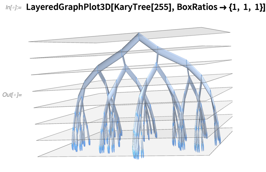
In Version 12.3 we’ve continued to expand that functionality. Here, for example, is a new 3D visualization function for graphs:

&#10005 LayeredGraphPlot3D[KaryTree[255], BoxRatios -> {1, 1, 1}]

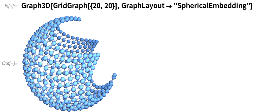
And here’s a new 3D graph embedding:

&#10005 Graph3D[GridGraph[{20, 20}], GraphLayout -> "SphericalEmbedding"]

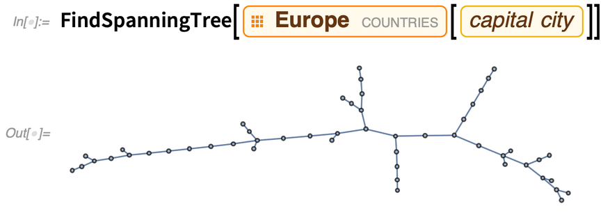
We’ve been able to find spanning trees in graphs since Version 10 (2014). In Version 12.3, however, we’ve generalized FindSpanningTree to directly handle objects—like geo locations—that have some kind of coordinates. Here’s a spanning tree based on the positions of capital cities in Europe:

&#10005 FindSpanningTree[ EntityClass["Country", "Europe"][ EntityProperty["Country", "CapitalCity"]]]

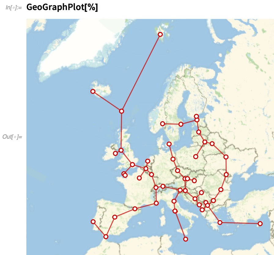
And now in Version 12.3 we can use the new GeoGraphPlot to plot this on a map:

&#10005 GeoGraphPlot[%]

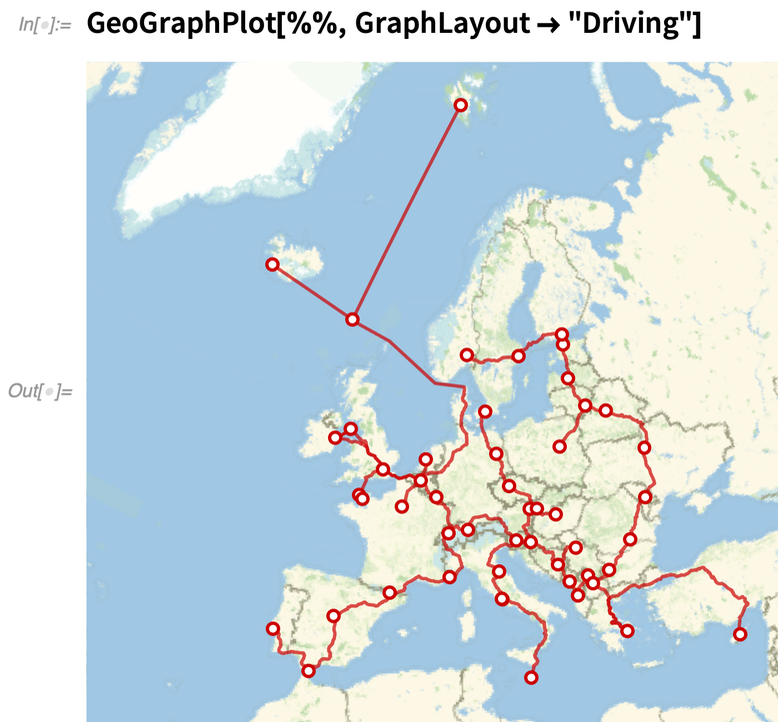
By the way, in a “geo graph” there are “geo” ways to route the edges. For example, you can specify that they follow (when possible) driving directions (as provided by TravelDirections):

&#10005 GeoGraphPlot[%%, GraphLayout -> "Driving"]

Graph Coloring (December 2021)

The graph theory capabilities of Wolfram Language have been very impressive for a long time (and were critical, for example, in making possible our Physics Project). But in Version 13.0 we’re adding still more.

A commonly requested set of capabilities revolve around graph coloring. For example, given a graph, how can one assign “colors” to its vertices so that no pair of adjacent vertices have the same color? In Version 13.0 there’s a function FindVertexColoring that does that:

&#10005

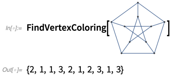
And now we can “highlight” the graph with those colors:

&#10005

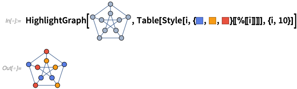
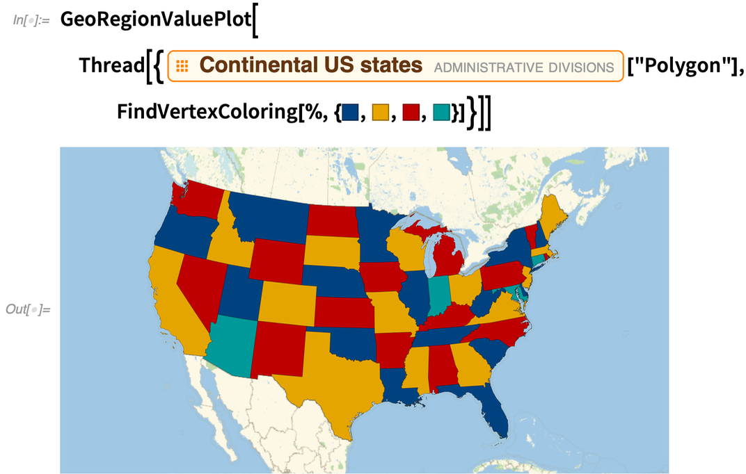
The classic “graph coloring” problem involves coloring geographic maps. So here, for example, is the graph representing the bordering relations for US states:

&#10005

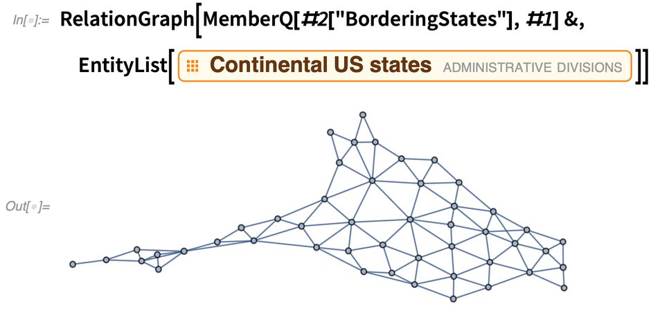
Now it’s an easy matter to find a 4-coloring of US states:

&#10005

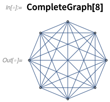
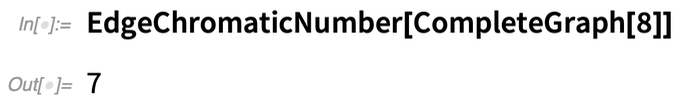
There are actually a remarkable range of problems that can be reduced to graph coloring. Another example has to do with scheduling a “tournament” in which all pairs of people “play” each other, but everyone plays only one match at a time. The collection of matches needed is just the complete graph:

&#10005

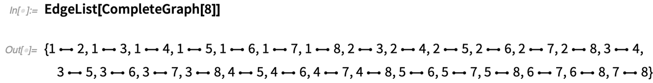
Each match corresponds to an edge in the graph:

&#10005

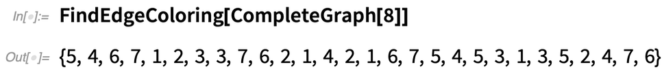
And now by finding an “edge coloring” we have a list of possible “time slots” in which each match can be played:

&#10005

EdgeChromaticNumber tells one the total number of matches needed:

&#10005

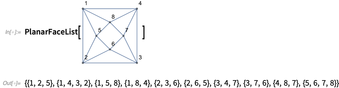
Map coloring brings up the subject of planar graphs. Version 13.0 introduces new functions for working with planar graphs. PlanarFaceList takes a planar graph and tells us how the graph can be decomposed into “faces”:

&#10005

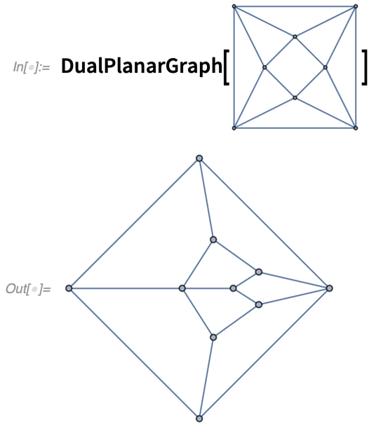
FindPlanarColoring directly computes a coloring for these planar faces. Meanwhile, DualPlanarGraph makes a graph in which each face is a vertex:

&#10005

Subgraph Isomorphism & More (December 2021)

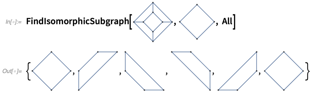
It comes up all over the place. (In fact, in our Physics Project it’s even something the universe is effectively doing throughout the network that represents space.) Where does a given graph contain a certain subgraph? In Version 13.0 there’s a function to determine that (the All says to give all instances):

&#10005

A typical area where this kind of subgraph isomorphism comes up is in chemistry. Here is the graph structure for a molecule:

&#10005

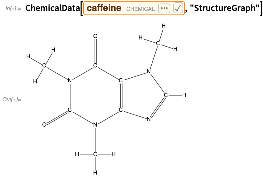
Now we can find a 6-cycle:

&#10005

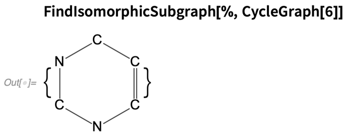
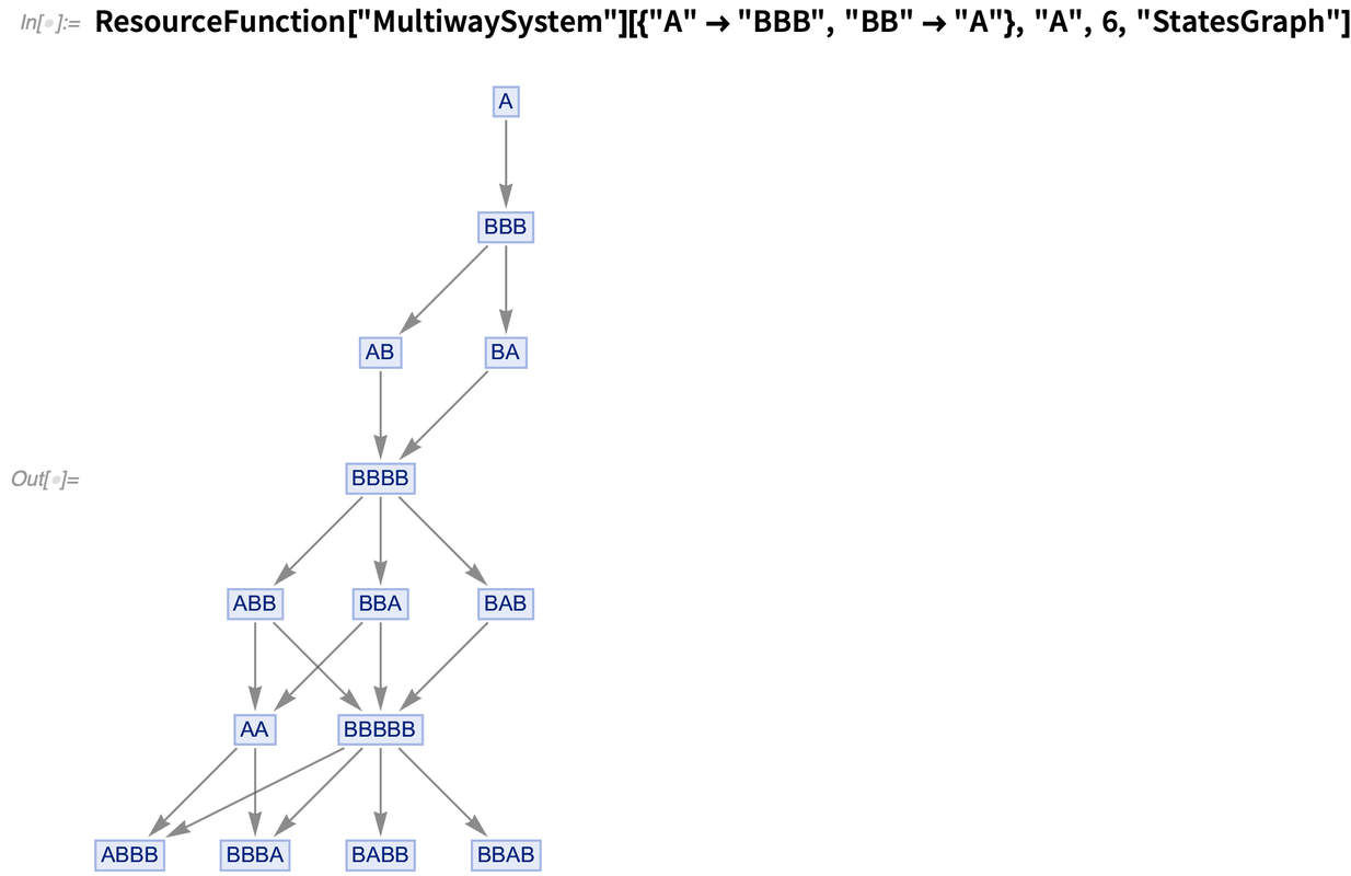
Another new capability in Version 13.0 has to do with handling flow graphs. The basic question is: in “flowing” through the graph, what vertices are critical, in the sense that they “have to be visited” if one’s going to get to all future vertices? Here’s an example of a directed graph (yes, made from a multiway system):

&#10005

Now we can ask for the DominatorTreeGraph, which shows us a map of what vertices are critical to reach where, starting from A:

&#10005

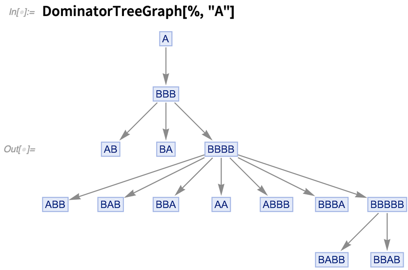
This now says for each vertex what its “dominator” is, i.e. what the nearest critical vertex to it is:

&#10005

If the graph represents causal or other dependency of one “event” on others, the dominators are effectively synchronization points, where everything has to proceed through one “thread of history”.

The Calculus of Annotations (March 2020)

How do you add metadata annotations to something you’re computing with? For Version 12.1 we’ve begun rolling out a general framework for making annotations—and then computing with and from them.

Let’s talk first about the example of graphs. You can have both annotations that you can immediately “see in the graph” (like vertex colors), and ones that you can’t (like edge weights).

Here’s an example where we’re explicitly constructing a graph with annotations:

&#10005 Graph[{Annotation[1 -> 2, EdgeStyle -> Red], Annotation[2 -> 1, EdgeStyle -> Blue]}]

Here we’re annotating the vertices:

&#10005 Graph[{Annotation[x, VertexStyle -> Red], Annotation[y, VertexStyle -> Blue]}, {x -> y, y -> x, y -> y}, VertexSize -> .2]

AnnotationValue lets you query values of annotations:

&#10005 AnnotationValue[{%, x}, VertexStyle]

Something important about AnnotationValue is that you can assign it. Set g to be the graph:

&#10005 g = CloudGet["https://wolfr.am/L9rgvixl"];

Now do an assignment to an annotation value:

&#10005 AnnotationValue[{g, x}, VertexStyle] = Green

Now the graph has changed:

&#10005 g

You can always delete the annotation if you want:

&#10005 AnnotationDelete[{g, x}, VertexStyle]

If you don’t want to permanently modify a graph, you can just use Annotate to produce a new graph with annotations added (3 and 5 are names of vertices):

&#10005 Annotate[{CloudGet["https://wolfr.am/L9rpqPJ0"], {3, 5}}, VertexSize -> .3]

Some annotations are important for actual computations on graphs. An example is edge weighting. This puts edge-weight annotations into a graph—though by default they don’t get displayed:

&#10005 Graph[Catenate[ Table[Annotation[i -> j, EdgeWeight -> GCD[i, j]], {i, 5}, {j, 5}]]]

This displays the edge weights:

&#10005 Graph[%, EdgeLabels -> "EdgeWeight"]

And this actually does a computation that includes the weights:

&#10005 WeightedAdjacencyMatrix[ CloudGet["https://wolfr.am/L9rtJdd9"]] // MatrixForm

You can use your own custom annotations too:

&#10005 Graph[{Annotation[x, "age" -> 10], Annotation[y, "age" -> 20]}, {x -> y, y -> x, y -> y}]

This retrieves the value of the annotation:

&#10005 AnnotationValue[{CloudGet["https://wolfr.am/L9rx8Mxe"], x}, "age"]

Annotations are ultimately stored in an AnnotationRules option:

&#10005 Options[CloudGet["https://wolfr.am/L9rx8Mxe"], AnnotationRules]

You can always give all annotations as a setting for this option.

A major complexity with annotations is when in a computation they should be preserved—or combined—and when they should be dropped. We always try to keep annotations whenever it makes sense:

&#10005 TransitiveReductionGraph[CloudGet["https://wolfr.am/L9rBdIZt"]]

Annotations are something quite general, that apply not only to graphs, but to an increasing number of other constructs too. But in Version 12.1 we’ve added something else that’s specific to graphs, and that handles a complicated case there. It has to do with multigraphs, i.e. graphs with multiple edges between the same vertices. Take the graph:

&#10005 Graph[{1 -> 2, 1 -> 2}]

How do you distinguish these two edges? It’s not a question of annotation; you actually want these edges to be distinct, just like the vertices in the graph are distinct. Well, in Version 12.1, you can give names (or “tags”) to edges, just like you give names to vertices:

&#10005 EdgeTaggedGraph[{1 -> 2, 1 -> 2} -> {a, b}]

In the edge list for this graph the edges are shown “tagged”:

&#10005 EdgeList[%]

The tags are part of the edge specification:

&#10005 InputForm[%]