Two years ago we released Version 12.0 of the Wolfram Language. Here are the updates in geometric computation since then, including the latest features in 13.0. The contents of this post are compiled from Stephen Wolfram’s Release Announcements for 12.1, 12.2, 12.3 and 13.0.

Euclidean Geometry Goes Interactive (December 2020)

One of the major advances in Version 12.0 was the introduction of a symbolic representation for Euclidean geometry: you specify a symbolic GeometricScene, giving a variety of objects and constraints, and the Wolfram Language can “solve” it, and draw a diagram of a random instance that satisfies the constraints. In Version 12.2 we’ve made this interactive, so you can move the points in the diagram around, and everything will (if possible) interactively be rearranged so as to maintain the constraints.

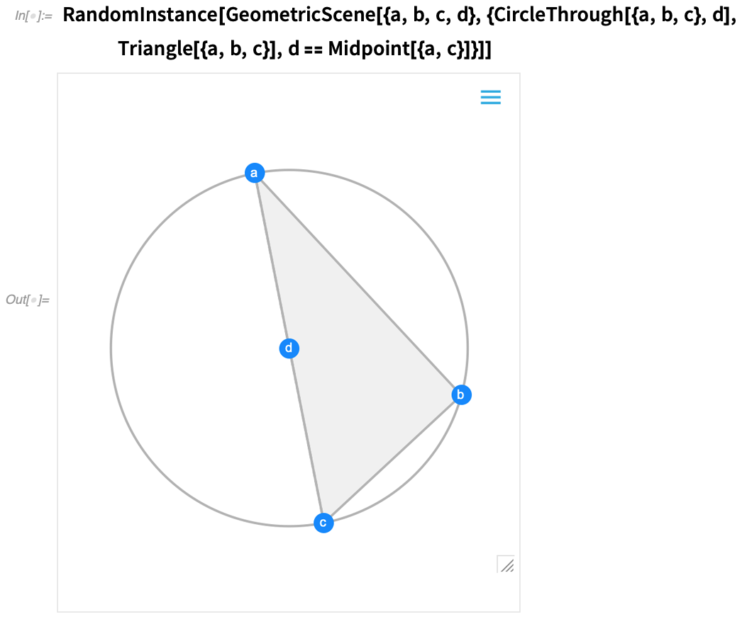
Here’s a random instance of a simple geometric scene:

&#10005 RandomInstance[ GeometricScene[{a, b, c, d}, {CircleThrough[{a, b, c}, d], Triangle[{a, b, c}], d == Midpoint[{a, c}]}]]

If you move one of the points, the other points will interactively be rearranged so as to maintain the constraints defined in the symbolic representation of the geometric scene:

&#10005 RandomInstance[ GeometricScene[{a, b, c, d}, {CircleThrough[{a, b, c}, d], Triangle[{a, b, c}], d == Midpoint[{a, c}]}]]

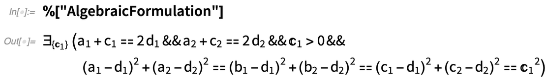
What’s really going on inside here? Basically, the geometry is getting converted to algebra. And if you want, you can get the algebraic formulation:

&#10005 %["AlgebraicFormulation"]

And, needless to say, you can manipulate this using the many powerful algebraic computation capabilities of the Wolfram Language.

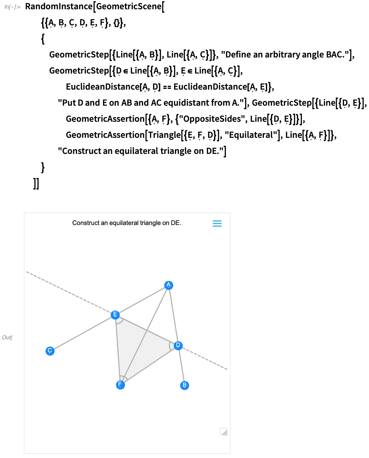
In addition to interactivity, another major new feature in 12.2 is the ability to handle not just complete geometric scenes, but also geometric constructions that involve building up a scene in multiple steps. Here’s an example—that happens to be taken directly from Euclid:

&#10005 RandomInstance[GeometricScene[ {{\[FormalCapitalA], \[FormalCapitalB], \[FormalCapitalC], \ \[FormalCapitalD], \[FormalCapitalE], \[FormalCapitalF]}, {}}, { GeometricStep[{Line[{\[FormalCapitalA], \[FormalCapitalB]}], Line[{\[FormalCapitalA], \[FormalCapitalC]}]}, "Define an arbitrary angle BAC."], GeometricStep[{\[FormalCapitalD] \[Element] Line[{\[FormalCapitalA], \[FormalCapitalB]}], \[FormalCapitalE] \ \[Element] Line[{\[FormalCapitalA], \[FormalCapitalC]}], EuclideanDistance[\[FormalCapitalA], \[FormalCapitalD]] == EuclideanDistance[\[FormalCapitalA], \[FormalCapitalE]]}, "Put D and E on AB and AC equidistant from A."], GeometricStep[{Line[{\[FormalCapitalD], \[FormalCapitalE]}], GeometricAssertion[{\[FormalCapitalA], \[FormalCapitalF]}, \ {"OppositeSides", Line[{\[FormalCapitalD], \[FormalCapitalE]}]}], GeometricAssertion[ Triangle[{\[FormalCapitalE], \[FormalCapitalF], \ \[FormalCapitalD]}], "Equilateral"], Line[{\[FormalCapitalA], \[FormalCapitalF]}]}, "Construct an equilateral triangle on DE."] } ]]

The first image you get is basically the result of the construction. And—like all other geometric scenes—it’s now interactive. But if you mouse over it, you’ll get controls that allow you to move to earlier steps:

&#10005

Move a point at an earlier step, and you’ll see what consequences that has for later steps in the construction.

Euclid’s geometry is the very first axiomatic system for mathematics that we know about. So—2000+ years later—it’s exciting that we can finally make it computable. (And, yes, it will eventually connect up with AxiomaticTheory, FindEquationalProof, etc.)

But in recognition of the significance of Euclid’s original formulation of geometry, we’ve added computable versions of his propositions (as well as a bunch of other “famous geometric theorems”). The example above turns out to be proposition 9 in Euclid’s book 1. And now, for example, we can get his original statement of it in Greek:

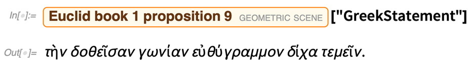
&#10005 Entity["GeometricScene", "EuclidBook1Proposition9"]["GreekStatement"]

And here it is in modern Wolfram Language—in a form that can be understood by both computers and humans:

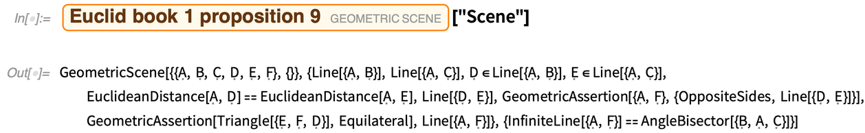
&#10005 Entity["GeometricScene", "EuclidBook1Proposition9"]["Scene"]

Euclid Meets Descartes (May 2021)

We’ve been doing a lot with geometry in the past few years, and there’s more to come. In Version 12.0 we introduced “Euclid-style” synthetic geometry. In Version 12.3 we’re connecting to “Descartes-style” analytic geometry, converting geometric descriptions to algebraic formulas.

Given three symbolically specified points, GeometricTest can give the algebraic condition for them to be collinear:

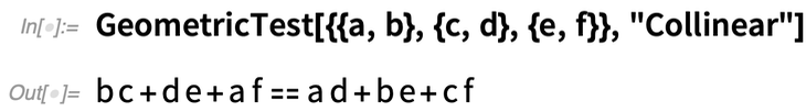
&#10005 GeometricTest[{{a, b}, {c, d}, {e, f}}, "Collinear"]

For the particular case of collinearity, there’s a specific function for doing the test:

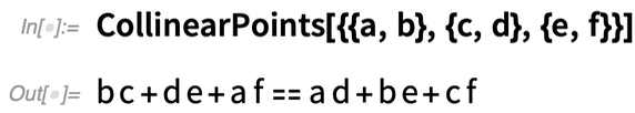
&#10005 CollinearPoints[{{a, b}, {c, d}, {e, f}}]

But GeometricTest is much more general in scope—supporting more than 30 kinds of predicates. This gives the condition for a polygon to be convex:

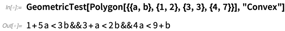
&#10005 GeometricTest[Polygon[{{a, b}, {1, 2}, {3, 3}, {4, 7}}], "Convex"]

And this gives the condition for a polygon to be regular:

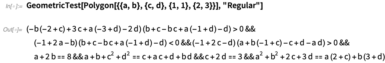
&#10005 GeometricTest[Polygon[{{a, b}, {c, d}, {1, 1}, {2, 3}}], "Regular"]

And here’s the condition for three circles to be mutually tangent (and, yes, that ∃ is a little “post Descartes”):

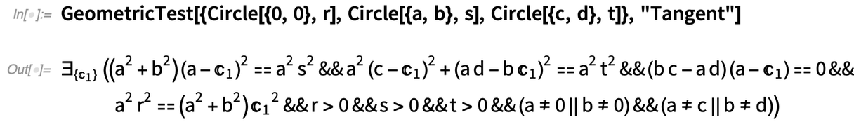
&#10005 GeometricTest[{Circle[{0, 0}, r], Circle[{a, b}, s], Circle[{c, d}, t]}, "Tangent"]

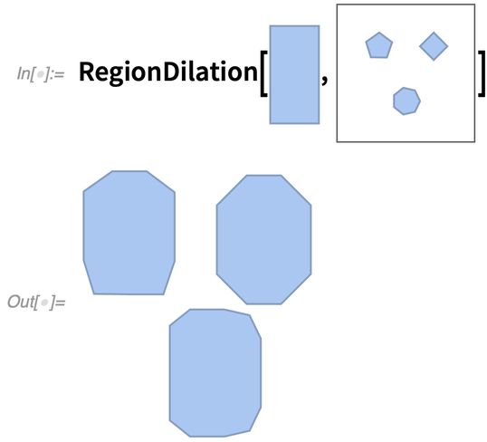
Version 12.3 also has enhancements to core computational geometry. Most notable are RegionDilation and RegionErosion, that essentially convolve regions with each other. RegionDilation effectively finds the whole (“Minkowski sum”) “union region” obtained by translating one region to every point in another region.

Why is this useful? It turns out there are lots of reasons. One example is the “piano mover problem” (AKA the robot motion planning problem). Given, say, a rectangular shape, is there a way to maneuver it (in the simplest case, without rotation) through a house with certain obstacles (like walls)?

Basically what you need to do is take the rectangular shape and “dilate the room” (and the obstacles) with it:

&#10005 RegionDilation[\!\(\* GraphicsBox[ TagBox[ DynamicModuleBox[{Typeset`mesh = HoldComplete[ BoundaryMeshRegion[{{0., 0.}, {0.11499999999999999`, 0.}, { 0.11499999999999999`, 0.22999999999999998`}, {0., 0.22999999999999998`}}, { Line[{{1, 2}, {2, 3}, {3, 4}, {4, 1}}]}, Method -> { "EliminateUnusedCoordinates" -> True, "DeleteDuplicateCoordinates" -> Automatic, "DeleteDuplicateCells" -> Automatic, "VertexAlias" -> Identity, "CheckOrientation" -> Automatic, "CoplanarityTolerance" -> Automatic, "CheckIntersections" -> Automatic, "BoundaryNesting" -> {{0, 0}}, "SeparateBoundaries" -> False, "TJunction" -> Automatic, "PropagateMarkers" -> True, "ZeroTest" -> Automatic, "Hash" -> 740210533488462839}]]}, TagBox[GraphicsComplexBox[{{0., 0.}, {0.11499999999999999`, 0.}, { 0.11499999999999999`, 0.22999999999999998`}, {0., 0.22999999999999998`}}, {Hue[0.6, 0.3, 0.95], EdgeForm[Hue[0.6, 0.3, 0.75]], TagBox[PolygonBox[{{1, 2, 3, 4}}], Annotation[#, "Geometry"]& ]}], MouseAppearanceTag["LinkHand"]], AllowKernelInitialization->False], "MeshGraphics", AutoDelete->True, Editable->False, Selectable->False], DefaultBaseStyle->{ "MeshGraphics", FrontEnd`GraphicsHighlightColor -> Hue[0.1, 1, 0.7]}, ImageSize->{27.866676879084963`, Automatic}]\), CloudGet["http://wolfr.am/VAs8Qsr5"]]

Then if there’s a connected path “left over” from one point to another, then it’s possible to move the piano along that path. (And of course, the same kind of thing can be done for robots in a factory, etc. etc.)

RegionDilation is also useful for “smoothing out” or “offsetting” shapes, for example, for CAD applications:

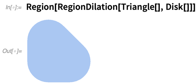
&#10005 Region[RegionDilation[Triangle[], Disk[]]]

At least in simple cases, one can “go Descartes” with it, and get explicit formulas:

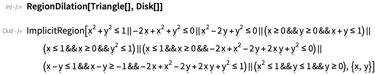
&#10005 RegionDilation[Triangle[], Disk[]]

And, by the way, this all works in any number of dimensions—providing a useful way to generate all sorts of “new shapes” (like a cylinder is the dilation of a disk by a line in 3D).

Geometric Regions: Fitting and Building (December 2021)

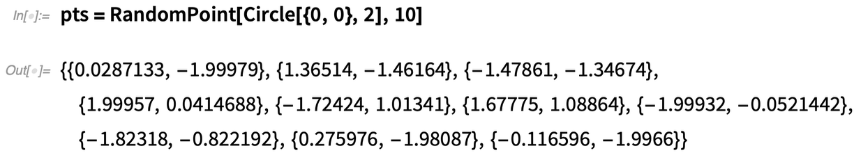
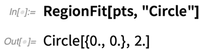
Given a bunch of points on a circle, what is the circle they are on?

Here are random points selected around a circle:

&#10005

The new function RegionFit can figure out what circle the points are on:

&#10005

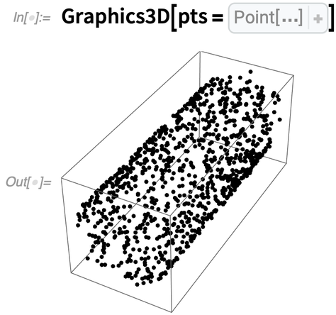
Here’s a collection of points in 3D:

&#10005

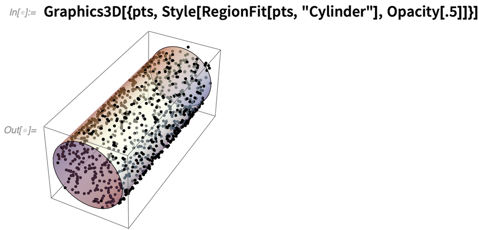
This fits a cylinder to these points:

&#10005

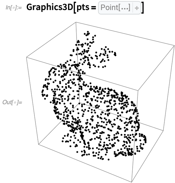
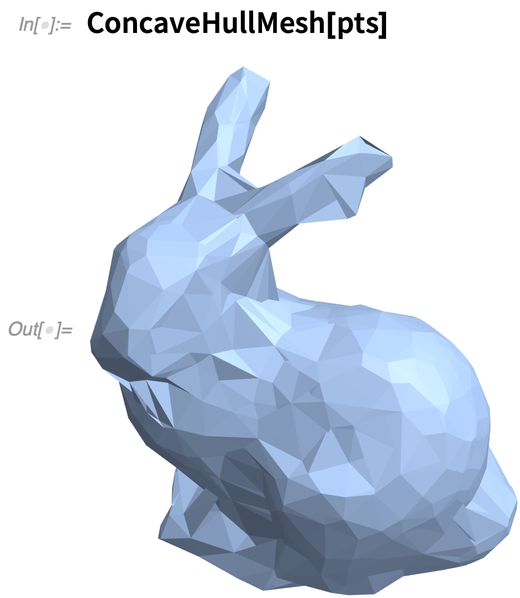
Another very useful new function in Version 13.0 is ConcaveHullMesh—which attempts to reconstruct a surface from a collection of 3D points. Here are 1000 points:

&#10005

The convex hull will put “shrinkwrap” around everything:

&#10005

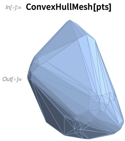
But the concave hull will make the surface “go into the concavities”:

&#10005

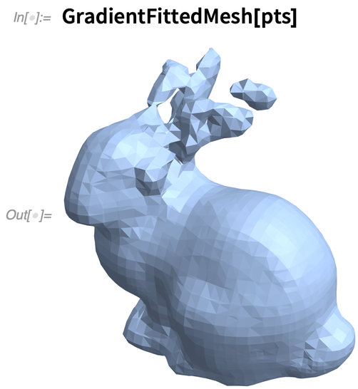
There’s a lot of freedom in how one can reconstruct the surface. Another function in Version 13 is GradientFittedMesh, which forms the surface from a collection of inferred surface normals:

&#10005

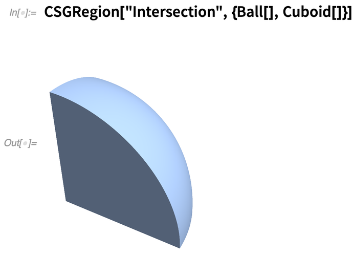
We’ve just talked about finding geometric regions from “point data”. Another new capability in Version 13.0 is constructive solid geometry (CSG), which explicitly builds up regions from geometric primitives. The main function is CSGRegion, which allows a variety of operations to be done on primitives. Here’s a region formed from an intersection of primitives:

&#10005

Note that this is an “exact” region—no numerical approximation is involved. So when we ask for its volume, we get an exact result:

&#10005

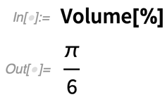
One can build up more complicated structures hierarchically:

&#10005

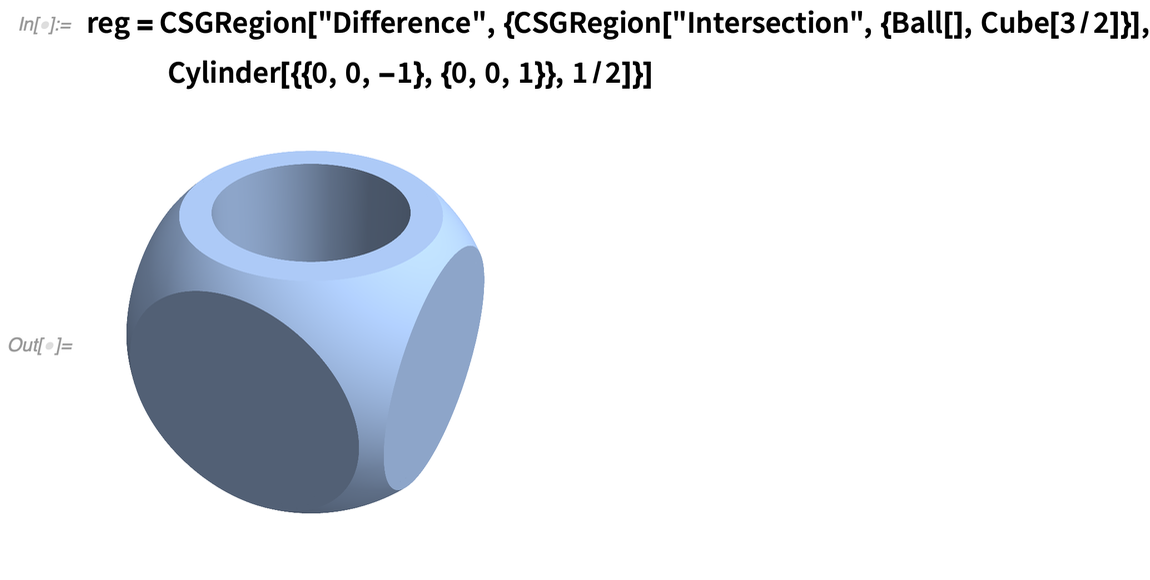
Though the integrals get difficult, it’s still often possible to get exact results for things like volume:

&#10005

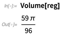
Given a hierarchically constructed geometric region, it’s possible to “tree it out” with CSGRegionTree:

&#10005

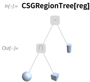
In doing mechanical engineering, it’s very common to make parts by physically performing various operations that can easily be represented in CSG form. So here for example is a slightly more complicated CSG tree

&#10005

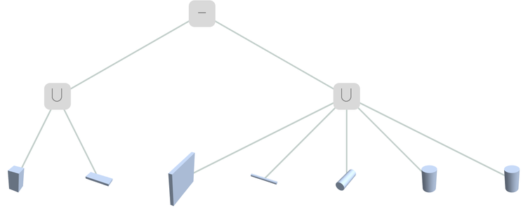
which can be “assembled” into an actual CSG region for a typical engineering part:

&#10005

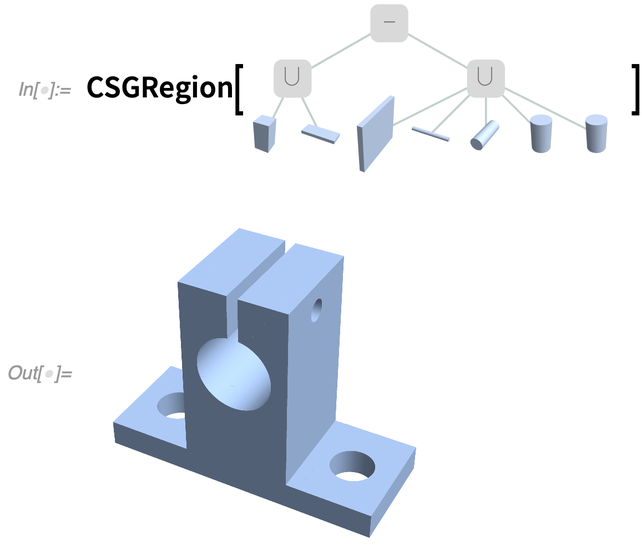
Thinking about CSG highlights the question of determining when two regions are “the same”. For example, even though a region might be represented as a general Polygon, it may actually also be a pure Rectangle. And more than that, the region might be at a different place in space, with a different orientation.

In Version 13.0 the function RegionCongruent tests for this:

&#10005

RegionSimilar also allows regions to change size:

&#10005

But knowing that two regions are similar, the next question might be: What transformation is needed to get from one to the other? In Version 13.0, FindRegionTransform tries to determine this:

&#10005

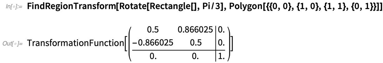
The Calculus of Annotations (March 2020)

How do you add metadata annotations to something you’re computing with? For Version 12.1 we’ve begun rolling out a general framework for making annotations—and then computing with and from them.

Another kind of structure that can be annotated just like graphs is a mesh. This is saying to annotate dimension-0 boundary cells with a style:

&#10005 Annotate[{MengerMesh[2], {0, "Boundary"}}, MeshCellStyle -> Red]