A Virtual Face-off: Replaying the 2020 Livecoding Championship
In early October, by what at this point can only be a time-honored tradition, the Livecoding Championship returned in its fifth annual iteration as a special event during the 2020 Wolfram Technology Conference. As in preceding years, the championship offered top Wolfram Language programmers a chance to show off their knowledge, agility, typing speed and documentation-reading skills to an unfailingly adoring audience.
Follow along with this post by watching this recorded video of the 2020 Livecoding Championship livestream!
The virtual setting of this year’s conference posed unique challenges for the competition, but our team took this as an opportunity to try a slightly different format for the event. Past competitors—and readers of last year’s recap blog—will remember that previous years’ questions were rigidly structured, with the judges expecting to see contestants’ code produce a specific, expected output for each. This year’s questions were much more open-ended and in many cases left purposely open to interpretation, allowing contestants to express both their creativity and humor alike. Our lively livestream audience was enlisted to judge, voting in real time on their favorite solutions out of the top five received for each question.
Audience favorite Flip Phillips and veteran livecoding contestant Philip Maymin reprised their roles as nominally overlapping MCs from the Wolfram Summer School competition earlier this year. Flip cohosted the 2019 event as well. This illustrious and industrious duo was also accorded the dubious privilege of question-writing, and I’m told they are still recovering.
In this post, I’ll walk our blog audience through this year’s competition questions and the top solutions received for each.

Question 1: “I Do Not Think It Means What You Think It Means”
Create a depiction of a mole using any Wolfram Language visualization functionality (e.g. symbolic graphics, graph plotting, equation plotting, etc.).
There are numerous possible moles to choose from here—the SI unit of amount of substance, the mammal, the tunnel-boring machine and probably about ![]() more. Let’s see which moles our contestants went for.
more. Let’s see which moles our contestants went for.
 Engage with the code in this post by downloading the Wolfram Notebook
First Place: Adereth

✕
Grid[ImageData[ImageResize[Binarize@Import["https://assets.dragoart.com/images/101719_502/how-to-draw-a-mole-for-kids-step-5_5e4c9ff3b14865.32843667_54930_3_3.gif"], 50]], Spacings -> 0] |
Adereth chose the mammalian option, downloading a line drawing of a mole from a website and converting it to a 50-pixel-wide bit matrix. An intellectual property court might have considered this a derivative work, but the court of public opinion awarded Adereth first place.
Second Place (Tied): Daniele Ceravolo

✕
WolframAlpha["mole curve"] |
At first glance, Daniele may appear simply to be querying the built-in popular curves data in Wolfram|Alpha for a parametric curve representing a superhero named “the Mole.” In fact, Daniele is querying the built-in popular curves data in Wolfram|Alpha for a parametric curve representing a superhero named “the Mole” created to represent the SI unit of amount of substance by a STEM outreach program of the US National Institute of Standards and Technology. Hence, presumably, the positive response by our always-knowledgeable livestream audience.
Second Place (Tied): Mike S


Mike S presents an intriguing machine learning–based solution, training a neural network to predict the color of each pixel in an image of a mole. The code Mike submitted is unfortunately incomplete, so we can’t see how the net was trained, but some amateur sleuthing turns up a suspiciously similar example from the documentation for the NetTrain function, demonstrated here with a different mole image.
Convert a test image into a training set, in which pixel positions (x, y) are mapped to color values (r, g, b):

✕
img = Entity["Species", "Family:Talpidae"][EntityProperty["Species", "Image"]] |

✕
dims = Reverse@ImageDimensions[img];rules = Flatten@MapIndexed[(2 (#2 - 1.)/(dims - 1) - 1.) -> #1 &, ImageData@img, {2}];
|

✕
RandomChoice[rules] |
Create a network to predict the color based on pixel position:

✕
chain = NetChain[{100, Ramp, 250, Ramp, 10, LogisticSigmoid, 3}]
|
Train the network:
|
✕
trained = NetTrain[chain, rules, MaxTrainingRounds -> 100]; |
Use the network to predict the entire original image:

✕
{h, v} = Range[-1, 1, 2./#] & /@ (dims);coords = Tuples[{h, v}];Image[Partition[trained@coords, Length[v]]]
|
Second Place (Tied): HP2000

✕
mol = MoleculePlot[Molecule["C"]]*6.02^23 |
HP2000 shows us a symbolic representation of (approximately) one mole of methane. It’s worth pointing out that a Molecule expression can be used for more than just generating pretty diagrams—a MoleculeValue can tell us that a mole of methane has a mass of about 16 grams, along with a host of other interesting properties of the molecule:

✕
Molecule["C"] |

✕
MoleculeValue[%, {"MolarMass", "ElementMassFraction", "Eccentricity"}]
|
Third Place: Total Annihilation

✕
Plot[PDF[CauchyDistribution[0, 1], x]^0.1, {x, -10, 10},
 PlotRange -> Full]
|
Total Annihilation captioned their solution “a cross-section of a skin tag.” No further elucidation is needed, I think.
Question 2: “The Most Ambiguous Word in the World”
Find the English word or words that are the most “ambiguous”—and yes, this question is itself ambiguous!
Let’s see what our contestants came up with in response to this vaguely self-congratulatory question.
First Place: Total Annihilation

✕
MaximalBy[WordData /@ WordData["*", "Lookup"], Length][[1, 1, 1]] |
Total Annihilation’s solution quite reasonably takes “most ambiguous” to mean “greatest number of definitions.” And “break” indeed has a whopping 76 definitions:

✕
WordData["break", "Definitions"] // Length |
Here’s just a sampling; check Wolfram|Alpha for the full list:

✕
Multicolumn[RandomSample[WordData["break", "Definitions"], 20],2,BaseStyle -> {Magnification -> .7}]
|
Second Place: Nik Murzin

✕
Select[WordList[], ContainsAll[Characters[#], Characters@"ambiguous"] &] |
Nik’s solution selects the English words that contain all the letters in the word “ambiguous.” Nik notes that their favorite of these is “bigamous”:

✕
WordDefinition["bigamous"] |
Substituting ContainsExactly for ContainsAll, we can see that “bigamous” is also the only other word containing exactly the same letters as “ambiguous”:

✕
Select[WordList[], ContainsExactly[Characters[#], Characters@"ambiguous"] &] |
Third Place: Wolfram Bob Repository

✕
{AbsoluteTiming[TakeLargestBy[WordList[], Length[WordDefinition[#]] &, 1]], ResourceFunction["BirdSay"]["Nice Answer Bob"]}
|
The curiously named contestant “Wolfram Bob Repository” (known to friends as “WBR”) uses a similar interpretation to Total Annihilation, with a BirdSay thrown in for good measure. Why, then, is WBR’s solution more than twice as fast as Total Annihilation’s (repeated below)?

✕
AbsoluteTiming[MaximalBy[WordData /@ WordData["*", "Lookup"], Length][[1, 1, 1]]] |
The answer lies in WBR’s obtaining a master list of words from the function WordList instead of WordData—the former is much smaller and is largely a subset of the latter:

✕
Length /@ {WordList[], WordData[]}
|
(Note that WordData[] is essentially equivalent to the form WordData["*","Lookup"] used by Total Annihilation.)
WordData contains many less-common words, particularly obscure compound words:

✕
RandomSample[Complement[WordData[], WordList[]], 20] |
Total Annihilation’s solution is much faster when iterating over the shorter WordList dictionary. In fact, it’s even faster than WBR’s version:

✕
AbsoluteTiming[MaximalBy[WordData /@ WordList[], Length][[1, 1, 1]]] |
This is because WBR uses the code WordDefinition["word"] to get a list of textual definitions for each word, while Total Annihilation uses WordData["word"]. The latter returns a list of word senses, each corresponding to a definition, and is about two times faster:

✕
Short[WordDefinition["break"], 3] // RepeatedTimingShort[WordData["break"], 3] // RepeatedTiming |
WordData can be used to get the definition of a given word sense:

✕
WordData[{"break", "Verb", "Ruin"}, "Definitions"]
|
Fourth Place (Tied): Hakan K

✕
SemanticInterpretation["ambigous", AmbiguityFunction -> All] |
Hakan K’s solution wittily makes use of the AmbiguityFunction option to the Interpreter and SemanticInterpretation functions. These functions interpret free-form text with natural language processing technology similar to that used by Wolfram|Alpha:

✕
SemanticInterpretation["wolfram"] |
The AmbiguityFunction option tells these functions how to handle multiple ambiguous results. The default setting is Automatic, which tells the function to simply return the first result. By specifying AmbiguityFunction → All, we ask instead for a list of all possible interpretations:

✕
SemanticInterpretation["wolfram", AmbiguityFunction -> All] |
In the case of the string “ambiguous,” we got two different results: an entity representing the word and another representing a MathWorld topic:

✕
SemanticInterpretation["ambigous", AmbiguityFunction -> All] |
|
✕
% // InputForm |
![]()
![]()
Fourth Place (Tied): Mike S

✕
wd = WordData[];First[ReverseSortBy[# -> Length[WordDefinition[#]] & /@ wd, Last]] |
Mike S takes the same interpretation as Total Annihilation and WBR, with the inclusion of a helpful count of the number of definitions associated with the winning word.
Question 3: “30-for-30”
Generate “30” using cellular automaton rule 30.
This question invites us to derive the number 30, or some variation thereof, from the rule 30 elementary cellular automaton.
First Place: Robert Mendelsohn

✕
c = Flatten@DeleteCases[WebImageSearch["rule 30 shell", "Images", MaxItems -> 30], $Failed]; ImageCollage[ConformImages[c[[1 ;; Length[c]]]]] |
Robert uses the WebImageSearch function to obtain up to 30 images corresponding to the query “rule 30 shell” (in reference to the cellular automaton–like pigmentation patterns found on some mollusc shells). WebImageSearch curiously returned only seven distinct images here, not the 30 Robert requested, as can be seen more clearly with borders around each image:

✕
ImageCollage[ImagePad[#, 5, Red] & /@ ConformImages[c[[1 ;; Length[c]]]]] |
The voting audience seemed to agree that in competition, it’s the thought that counts.
Second Place: Wolfram Bob Repository

✕
{Style["Click Me", 40],Table[ResourceFunction["DynamicCellularAutomaton"][30, {i, 30}], {i, 30}]}
|
WBR uses the DynamicCellularAutomaton resource function to create 30 interactive plots of rule 30, each 30 columns wide and showing up to 30 rows. Each plot can be clicked to edit the initial conditions in the first row.
Third Place: Mike S

✕
Total[CellularAutomaton[30, {0, 0, 0, 1, 0, 0, 0}, 9], 3]
|
Mike evolves rule 30 on a fixed seven-column grid and finds that the number of black cells on the grid after nine steps totals to 30. Nice and simple!

✕
CellularAutomaton[30, {0, 0, 0, 1, 0, 0, 0}, 9] // ArrayPlot
|
Fourth Place: Nik Murzin

✕
ResourceFunction["LogoQRCode"]["thirty", Rasterize@ArrayPlot[CellularAutomaton[30, {{1}, 0}, 50]]]
|
Nik uses the LogoQRCode resource function to create a QR code for the string “thirty,” with the center of the barcode containing a plot of rule 30. Leave your phone in your pocket; we can easily verify the contents of the barcode with BarcodeRecognize:

✕
BarcodeRecognize[%] |
Fifth Place: HP2000

✕
img = ArrayPlot[CellularAutomaton[30, {{1}, 0}, 30]]; GeoGraphics[{GeoStyling["OutlineMap", PatternFilling[img, {85, 48}]], Polygon[Entity["Country", "UnitedStates"]]}]
|
HP2000 shows us a map of the United States, tiled over with array plots of rule 30. It’s unclear where “30” appears in this visualization, as there are fewer than 30 copies of the plot. Perhaps HP2000 intends the map to depict the US in the period from May 29, 1848, to September 9, 1850, during which the country consisted of 30 states.
Question 4: “WWWD: What Would Wolfram Do?”
Write a function that will give the user advice on any yes/no question, based on both geolocation and current time.
The Wolfram Language does not yet have built-in divination functionality, so contestants were left to implement their own. Let’s see how they did.
First Place: Sander

✕
SeedRandom[StringJoin[ToString /@ {Here, Now}]]; Row@{ResourceFunction["PlayingCardGraphic"][RandomInteger[{1, 52}]], " which means ", RandomChoice[{"Yes", "No"}]}
|
Sander seeds the Wolfram Language random number generator with the user’s current spatiotemporal coordinates (taking stock of the Here and Now, so to speak), draws a card (using the PlayingCardGraphic resource function) and associates it with a yes/no answer. A careful reader might notice that nothing in Sander’s code guarantees that each card will always be paired with the same yes/no value, and indeed, one can elicit a contradiction after a few dozen tries:

✕
SeedRandom[StringJoin[ToString /@ {Here, Now}]]; Row@{ResourceFunction["PlayingCardGraphic"][RandomInteger[{1, 52}]], " which means ", RandomChoice[{"Yes", "No"}]}
|
But nothing in the question mandated that solutions produce rational output, and in my experience, oracles rarely do.
Second Place: Robert Mendelsohn

✕
ListAnimate[Table[ImageRestyle[Rasterize[{DateString[], InputField["What do you need help with?"],InputField["Where are you located?"]}], w -> Rasterize[{WebImageSearch["Starry Night"], Table[RandomWord[], {20}]}]], {w, 0, 1, 0.2}]]
|
Robert’s solution is elaborate and mystifying. It starts by creating an image based on the current date and a pair of InputField expressions:

✕
Rasterize[{DateString[], InputField["What do you need help with?"], InputField["Where are you located?"]}]
|
It’s unclear why Robert is using InputField here. They may have intended instead to use Input, in order to prompt the user with a dialog box:

✕
img1 = Rasterize[{DateString[], Input["What do you need help with?"], Input["Where are you located?"]}]
|
Robert then searches the web for some images of van Gogh’s The Starry Night, and picks 20 random dictionary words. These too are rasterized into a single image:

✕
img2 = Rasterize[{WebImageSearch["Starry Night"], Table[RandomWord[], {20}]}]
|
Finally, the ImageRestyle function is used to transfer the style of the second image (The Starry Night and the words) onto the first (date and user inputs) using machine learning. This is done six times, with different weighting each time, producing an eerie slideshow:

✕
ListAnimate[Table[ImageRestyle[img1, w -> img2, TargetDevice -> "GPU"], {w, 0, 1, 0.2}]]
|
Interpretation of this result is an exercise left to the reader.
Third Place: Nik Murzin

✕
If[Mod[Mean[First@Here] + DateValue[Now, "SecondExact"], 2] < 0, "Yes", "No"] |
Nik’s solution performs some arithmetic based on the user’s latitude and longitude and the number of fractional seconds elapsed in the current minute. The results are rather pessimistic:

✕
Table[Block[{Now = FromAbsoluteTime[RandomReal[10^12]]},If[Mod[Mean[First@Here] + DateValue[Now, "SecondExact"], 2] < 0, "Yes", "No"]], 100]
|
Nik’s code has the test Mod[x,2]<0. The return value of Mod given these arguments is always non-negative, so the test will always return False:

✕
Plot[Mod[x, 2], {x, -5, 5}]
|
Nik is well within his rights to make a philosophical statement here, but those in the glass-not-totally-empty crowd may wish to change the test to Mod[...]<1 for a more balanced output:
 
✕
Table[Block[{Now = FromAbsoluteTime[RandomReal[10^12]]},If[Mod[Mean[First@Here] + DateValue[Now, "SecondExact"], 2] < 1, "Yes", "No"]], 100]% // Counts
|
Fourth Place: Total Annihilation

✕
If[EvenQ[Hash[{$GeoLocation, Now}]], "Yes", "No"]
|
Total Annihilation’s solution succinctly calculates an integer hash of the user’s location and the current timestamp and checks whether the result is even:

✕
Table[Block[{Now = FromAbsoluteTime[RandomReal[10^12]]},If[EvenQ[Hash[{$GeoLocation, Now}]], "Yes", "No"]], 10000] // Counts
|
Fifth Place: Adereth

✕
{"As I see it, yes.", "Ask again later.", "Better not tell you now.", "Cannot predict now.", "Concentrate and ask again.", "Don't count on it.", "It is certain.", "It is decidedly so."}[[1 + Mod[Hash@{GeoLocation[], Now}, 8]]]
|
Adereth goes the extra mile and includes a set of Magic 8-Ball answers for some extra dimension. They use a similar approach to Total Annihilation, basing the result on a hash of the user’s location and the present time.
Question 5: “Eye Find the Settings Optical”
Generate or replicate an optical illusion. These might get you started on getting an idea for your illusions: Wolfram|Alpha illusions search, the Illusions Index, eyetricks.net and Illusion of the Year.
First Place: Nik Murzin

✕
animateCircle[n_] := Animate[Graphics[Flatten@{Disk[], White, Map[(phase = #*2 \[Pi]/n;line = {Cos[phase], Sin[phase]};{Line[{-line, line}], Disk[Sin[t + phase]*line, 0.05]}) &, Range[n]]}, PlotRange -> {{-1.1, 1.1}, {-1.1, 1.1}}], {t, 0, 2 \[Pi]}]animateCircle[15]
|
Nik’s illusion demonstrates cycloid motion, wherein a set of points moving in phased sinusoidal motion along the diameter lines of a large circle trace out a smaller circle. We can examine how the effect is constructed by changing the number of visible points:

✕
Manipulate[With[{n = 15},Animate[Graphics[Flatten@{Disk[], White, Map[(phase = #*2 \[Pi]/n;line = {Cos[phase], Sin[phase]};{Line[{-line, line}], Disk[Sin[t + phase]*line, 0.05]}) &, Range[points]]}, PlotRange -> {{-1.1, 1.1}, {-1.1, 1.1}}], {t, 0, 2 \[Pi]}]],{points, 1, 15, 1}]
|
Second Place: Robert Mendelsohn

✕
Manipulate[Graphics[{
   {If[layer1, {Rotate[
       Scale[Table[
         Rotate[{If[show, {c, Rectangle[{0, 0}, {.6, 1}]}, {}],
           {y, Scale[Disk[{0, .5}, .3], {.9, 1.67}]},
           {z, Scale[Disk[{.6, .5}, .3], {.9, 1.67}]}},
          x, {0.3, -3}], {x, 0, 2 Pi, Pi/9}], 1.78], 0]}, {}]},
   Sequence[{
If[layer2, {
Rotate[
Scale[
Table[
Rotate[{
If[show, {c,
Rectangle[{0, 0}, {0.6, 1}]}, {}], {y,
Scale[
Disk[{0, 0.5}, 0.3], {0.9, 1.67}]}, {z,
Scale[
Disk[{0.6, 0.5}, 0.3], {0.9, 1.67}]}}, x, {0.3, -3}], {
          x, 0, 2 Pi, Pi/9}], 1.335], Pi/6]}, {}]}, {
Table[
Rotate[{
If[show, {c,
Rectangle[{0, 0}, {0.6, 1}]}, {}], {y,
Scale[
Disk[{0, 0.5}, 0.3], {0.9, 1.67}]}, {z,
Scale[
Disk[{0.6, 0.5}, 0.3], {0.9, 1.67}]}}, x, {0.3, -3}], {
      x, 0, 2 Pi, Pi/9}]}, {
Rotate[
Scale[
Table[
Rotate[{
If[show, {c,
Rectangle[{0, 0}, {0.6, 1}]}, {}], {y,
Scale[
Disk[{0, 0.5}, 0.3], {0.9, 1.67}]}, {z,
Scale[
Disk[{0.6, 0.5}, 0.3], {0.9, 1.67}]}}, x, {0.3, -3}], {
        x, 0, 2 Pi, Pi/9}], 0.75], Pi/6]}, {
Rotate[
Scale[
Table[
Rotate[{
If[show, {c,
Rectangle[{0, 0}, {0.6, 1}]}, {}], {y,
Scale[
Disk[{0, 0.5}, 0.3], {0.9, 1.67}]}, {z,
Scale[
Disk[{0.6, 0.5}, 0.3], {0.9, 1.67}]}}, x, {0.3, -3}], {
        x, 0, 2 Pi, Pi/9}], 0.56], 0]}, {
Rotate[
Scale[
Table[
Rotate[{
If[show, {c,
Rectangle[{0, 0}, {0.6, 1}]}, {}], {y,
Scale[
Disk[{0, 0.5}, 0.3], {0.9, 1.67}]}, {z,
Scale[
Disk[{0.6, 0.5}, 0.3], {0.9, 1.67}]}}, x, {0.3, -3}], {
        x, 0, 2 Pi, Pi/9}], 0.42], Pi/6]}, {
Rotate[
Scale[
Table[
Rotate[{
If[show, {c,
Rectangle[{0, 0}, {0.6, 1}]}, {}], {y,
Scale[
Disk[{0, 0.5}, 0.3], {0.9, 1.67}]}, {z,
Scale[
Disk[{0.6, 0.5}, 0.3], {0.9, 1.67}]}}, x, {0.3, -3}], {
        x, 0, 2 Pi, Pi/9}], 0.315], 0]}, {
Rotate[
Scale[
Table[
Rotate[{
If[show, {c,
Rectangle[{0, 0}, {0.6, 1}]}, {}], {y,
Scale[
Disk[{0, 0.5}, 0.3], {0.9, 1.67}]}, {z,
Scale[
Disk[{0.6, 0.5}, 0.3], {0.9, 1.67}]}}, x, {0.3, -3}], {
        x, 0, 2 Pi, Pi/9}], 0.235], Pi/6]}, {
Rotate[
Scale[
Table[
Rotate[{
If[show, {c,
Rectangle[{0, 0}, {0.6, 1}]}, {}], {y,
Scale[
Disk[{0, 0.5}, 0.3], {0.9, 1.67}]}, {z,
Scale[
Disk[{0.6, 0.5}, 0.3], {0.9, 1.67}]}}, x, {0.3, -3}], {
        x, 0, 2 Pi, Pi/9}], 0.1755], 0]}, {
Rotate[
Scale[
Table[
Rotate[{
If[show, {c,
Rectangle[{0, 0}, {0.6, 1}]}, {}], {y,
Scale[
Disk[{0, 0.5}, 0.3], {0.9, 1.67}]}, {z,
Scale[
Disk[{0.6, 0.5}, 0.3], {0.9, 1.67}]}}, x, {0.3, -3}], {
        x, 0, 2 Pi, Pi/9}], 0.132], Pi/6]}],
   {Black, Disk[{0.3, -3}, 0.45]},
   {White, FontSize -> 12, Text["A", {0.34, -3}]},
   {If[hide, {},
     {{If[
        layer1, {Rotate[
          Scale[Table[
            Rotate[{If[show, {c, Rectangle[{15, 0}, {15.6, 1}]}, {}],
              {y, Scale[Disk[{15, .5}, .3], {.9, 1.67}]},
              {z, Scale[Disk[{15.6, .5}, .3], {.9, 1.67}]}},
             x, {15.3, -3}], {x, 0, 2 Pi, Pi/9}], 1.78], 0]}, {}]},
      Sequence[{
If[layer2, {
Rotate[
Scale[
Table[
Rotate[{
If[show, {c,
Rectangle[{15, 0}, {15.6, 1}]}, {}], {y,
Scale[
Disk[{15, 0.5}, 0.3], {0.9, 1.67}]}, {z,
Scale[
Disk[{15.6, 0.5}, 0.3], {0.9, 1.67}]}}, x, {15.3, -3}], {
             x, 0, 2 Pi, Pi/9}], 1.335], Pi/6]}, {}]}, {
Table[
Rotate[{
If[show, {c,
Rectangle[{15, 0}, {15.6, 1}]}, {}], {y,
Scale[
Disk[{15, 0.5}, 0.3], {0.9, 1.67}]}, {z,
Scale[
Disk[{15.6, 0.5}, 0.3], {0.9, 1.67}]}}, x, {15.3, -3}], {
         x, 0, 2 Pi, Pi/9}]}, {
Rotate[
Scale[
Table[
Rotate[{
If[show, {c,
Rectangle[{15, 0}, {15.6, 1}]}, {}], {y,
Scale[
Disk[{15, 0.5}, 0.3], {0.9, 1.67}]}, {z,
Scale[
Disk[{15.6, 0.5}, 0.3], {0.9, 1.67}]}}, x, {15.3, -3}], {
           x, 0, 2 Pi, Pi/9}], 0.75], Pi/6]}, {
Rotate[
Scale[
Table[
Rotate[{
If[show, {c,
Rectangle[{15, 0}, {15.6, 1}]}, {}], {y,
Scale[
Disk[{15, 0.5}, 0.3], {0.9, 1.67}]}, {z,
Scale[
Disk[{15.6, 0.5}, 0.3], {0.9, 1.67}]}}, x, {15.3, -3}], {
           x, 0, 2 Pi, Pi/9}], 0.56], 0]}, {
Rotate[
Scale[
Table[
Rotate[{
If[show, {c,
Rectangle[{15, 0}, {15.6, 1}]}, {}], {y,
Scale[
Disk[{15, 0.5}, 0.3], {0.9, 1.67}]}, {z,
Scale[
Disk[{15.6, 0.5}, 0.3], {0.9, 1.67}]}}, x, {15.3, -3}], {
           x, 0, 2 Pi, Pi/9}], 0.42], Pi/6]}, {
Rotate[
Scale[
Table[
Rotate[{
If[show, {c,
Rectangle[{15, 0}, {15.6, 1}]}, {}], {y,
Scale[
Disk[{15, 0.5}, 0.3], {0.9, 1.67}]}, {z,
Scale[
Disk[{15.6, 0.5}, 0.3], {0.9, 1.67}]}}, x, {15.3, -3}], {
           x, 0, 2 Pi, Pi/9}], 0.315], 0]}, {
Rotate[
Scale[
Table[
Rotate[{
If[show, {c,
Rectangle[{15, 0}, {15.6, 1}]}, {}], {y,
Scale[
Disk[{15, 0.5}, 0.3], {0.9, 1.67}]}, {z,
Scale[
Disk[{15.6, 0.5}, 0.3], {0.9, 1.67}]}}, x, {15.3, -3}], {
           x, 0, 2 Pi, Pi/9}], 0.235], Pi/6]}, {
Rotate[
Scale[
Table[
Rotate[{
If[show, {c,
Rectangle[{15, 0}, {15.6, 1}]}, {}], {y,
Scale[
Disk[{15, 0.5}, 0.3], {0.9, 1.67}]}, {z,
Scale[
Disk[{15.6, 0.5}, 0.3], {0.9, 1.67}]}}, x, {15.3, -3}], {
           x, 0, 2 Pi, Pi/9}], 0.1755], 0]}, {
Rotate[
Scale[
Table[
Rotate[{
If[show, {c,
Rectangle[{15, 0}, {15.6, 1}]}, {}], {y,
Scale[
Disk[{15, 0.5}, 0.3], {0.9, 1.67}]}, {z,
Scale[
Disk[{15.6, 0.5}, 0.3], {0.9, 1.67}]}}, x, {15.3, -3}], {
           x, 0, 2 Pi, Pi/9}], 0.132], Pi/6]}],
      {Black, Disk[{15.3, -3}, 0.45]},
      {White, FontSize -> 12, Text["B", {15.38, -3}]}}]}
   }, ImageSize -> 600, PlotRange -> {{-7, 23}, {-11, 5}}],
 Row[{Control[{{y, Blue, "left color"}, {Red, Orange, Yellow, Green,
      Blue, Purple}}], Spacer[30],
   Control[{{z, Yellow, "right color"}, {Red, Orange, Yellow, Green,
      Blue, Purple}}], Spacer[30],
   Control[{{show, True, "show hourglass"}, {True, False}}],
   Spacer[30],
   Control[{{c, Black, "hourglass color"}, {Black, Gray, Brown,
      Red}}]}],
 Row[{Control[{{layer1, True, "show outside layer"}, {True, False}}],
   Spacer[30],
   Control[{{layer2, True, "show next layer"}, {True, False}}],
   Spacer[30],
   Control[{{hide, False, "hide second figure"}, {True, False}}]}],
 ContentSize -> {620, 340}
 ]
|
Robert’s highly elaborate solution creates the “rotating snakes” illusion—stare at the center of one circle and the outer rings appear to move.
Third Place: Sander

✕
Graphics[Table[{Pink, Disk[{x, y}, 0.4], Thickness[0.01], Black,
   Circle[{x, y}, 0.4, {(x + y) Pi/4, (x + y) Pi/4 + Pi}], White,
   Circle[{x, y}, 0.4, {(x + y) Pi/4 + Pi, (x + y) Pi/4 + 2 Pi}]}, {x,
    0, 15}, {y, 0, 15}], Background -> Darker[Yellow, 0.1]]
|
Sander’s solution is another peripheral drift illusion, similar to the rotating snakes.
Fourth Place: Adereth

✕
With[{n = 150},ArrayPlot[Table[Mod[i*j, n], {i, n}, {j, n}],ColorFunction -> "Rainbow"]]
|
Adereth has produced a discrete Cartesian plot where the value of each point is the product of its coordinates modulo the plot range. Symmetry emerges when the function is plotted discretely in the integer domain, but a continuous plot reveals it as “illusory”:

✕
With[{n = 15},DensityPlot[Mod[i*j, n], {i, 1, n}, {j, 1, n},ColorFunction -> "Rainbow",PlotLegends -> Automatic,Mesh -> n - 2,Exclusions -> None,PlotPoints -> 100]]
|
This author notes some interesting patterns reminiscent of “magic eye” autostereograms to be had by changing ![]() to
to ![]() :
:
 
✕
With[{n = 150},
 Manipulate[
  ArrayPlot[
   Table[Mod[i^j, m], {i, n}, {j, n}],
   ColorFunction -> "Rainbow",
   PlotLegends -> Automatic
   ],
  {{m, n}, 1, n, 1}
  ]]
|
Fifth Place: Mike S

✕
Manipulate[
 Graphics[{Black,
    Table[Rectangle[{x, y}, {x + 1, y + 1}], {x, 0, 20, 2}, {y, 0, 19,
       2}], Table[
     Rectangle[{x + 1, y + 1}, {x + 2, y + 2}], {x, 0, 19, 2}, {y, 0,
      17, 2}], GrayLevel[1 - gl], ,
    Table[{If[x == 2, {}, Disk[{x + .15, y + .15}, .15]],
      Disk[{x + .85, y + .85}, .15]}, {x, 2, 8, 2}, {y, 4, 8, 2}],
    Table[{If[y == 2, {}, Disk[{x + 1.15, y + 1.15}, .15]],
      Disk[{x + If[y == 8, 1.15, 1.85], y + 1.85}, .15]}, {x, 2, 8,
      2}, {y, 2, 8, 2}],

    Table[{Disk[{x + .15, y + If[x == 10, .15, .85]}, .15],
      If[x == 18, {}, Disk[{x + .85, y + .15}, .15]]}, {x, 10, 18,
      2}, {y, 4, 8, 2}],
    Table[{If[y == 2, {}, Disk[{x + 1.85, y + 1.15}, .15]],
      Disk[{x + If[y == 8, 1.85, 1.15], y + 1.85}, .15]}, {x, 10, 17,
      2}, {y, 2, 8, 2}],

    Table[{Disk[{x + .85, y + .15}, .15],
      If[x == 2, {}, Disk[{x + .15, y + .85}, .15]]}, {x, 2, 8,
      2}, {y, 10, 15, 2}],
    Table[{If[y == 14, {}, Disk[{x + 1.15, y + 1.85}, .15]],
      Disk[{x + 1.85, y + 1.15}, .15]}, {x, 2, 8, 2}, {y, 10, 15,
      2}],

    Table[{Disk[{x + .15, y + If[x == 10, .85, .15]}, .15],
      If[x == 18, {}, Disk[{x + .85, y + .85}, .15]]}, {x, 10, 18,
      2}, {y, 10, 15, 2}],
    Table[{Disk[{x + 1.15, y + 1.15}, .15],
      If[y == 14, {}, Disk[{x + 1.85, y + 1.85}, .15]]}, {x, 10, 17,
      2}, {y, 10, 15, 2}],

    Table[{Disk[{x + 1.85, 8 + 1.5}, .15]}, {x, 2, 8, 2}],
    Table[{Disk[{x + 1.15, 8 + 1.5}, .15]}, {x, 10, 16, 2}]} /.
   If[figure == "disks", {},
    Disk[c_, r_] -> Rectangle[c - r/2, c + r/2]],
  ImageSize -> 480], {{gl, .1, "gray level"}, 1,
  0}, {figure, {"disks", "squares"}}]
|
Mike’s solution is based on the code of the “warped squares” illusion from the Wolfram Demonstrations Project. The checkerboard squares appear to deform toward the center of the grid, but fading out the added disks with the “gray level” slider shows the grid to, in fact, be regular.
Question 6: “∀ Poetry: Rhyme || Reason”
Generate any kind of structured poem. It doesn’t have to make sense, but it does have to follow the right form.
The Wolfram Function Repository contains some poetically leaning resource functions, like WordWeave and RandomEnglishHaiku, but our contestants were instructed to create their solution from scratch. Let’s see what they came up with.
First Place: Sander

✕
w = WordData[];
w = Select[w, StringLength[#] > 5 &];
w = RandomSample /@ GatherBy[w, StringTake[#, -3] &];
w = RandomSample[w];
w = Select[w, Length[#] > 2 &];
{w[[1, 1]], w[[2, 1]], w[[1, 2]], w[[2, 2]], " ", w[[3, 1]],
  w[[4, 1]], w[[3, 2]], w[[4, 2]], " ", w[[5, 1]], w[[6, 1]],
  w[[5, 2]], w[[6, 2]], " ", w[[7, 1]], w[[7, 2]]} // Column
|
Sander generates a pseudo-Shakespearean sonnet, discarding the conventional syllabic scheme but retaining the rhyme pattern ABAB-CDCD-EFEF-GG. Determining whether two English words rhyme based solely on their spelling is a nontrivial task, but Sander’s quick-and-dirty approach to compare the final three letters of each word appears to work quite well in this case.
Second Place: Robert Mendelsohn

✕
{Module[{poetrynotes = Table[RandomInteger[{1, 24}], {17}]}, EmitSound[SoundNote[#, 1, "Piano"] & /@ poetrynotes]], "A tone poem for you"}
|
Robert creates a “tone poem” by stringing together random piano notes between C#4 and C6. The resulting composition may be the first piece in history eligible for a Pulitzer Prize in both music and poetry.
Third Place (Tied): Wolfram Bob Repository

✕
With[{w = RandomChoice[WordList[], 5]},
 Column[{
   StringRiffle[
    Flatten@{w, First[ResourceFunction["Rhymes"][#]] & /@ w}],
   ResourceFunction["PartyParrot"]["Dab", "SimpleAnimation"]
   }]
 ]
|
WBR describes this as a “poem with attitude.” The code picks five random words and uses the Rhymes resource function (by fellow contestant Mike S) to find other words that rhyme with each of the five original words. A distinctly hip parrot caps off the piece.
Third Place (Tied): Nik Murzin

✕
Column@Table[
  With[{s = IntegerName@RandomInteger[10]},
   RandomChoice@ResourceFunction["Rhymes"]@s], 10]
|
Nik creates an “integer poem” by finding rhymes for the English names of 10 random integers in the range ![]() . This is easier to understand if we pair each number with its rhyme:
. This is easier to understand if we pair each number with its rhyme:

✕
Grid@Table[
  With[{s = IntegerName@RandomInteger[10]}, {s,
    RandomChoice@ResourceFunction["Rhymes"]@s}], 10]
|
Third Place (Tied): Total Annihilation

✕
rhymes = GroupBy[WordData[],
   Replace[WordData[#, "PhoneticForm"],
     s_String :> Last[StringSplit[#, "'"]]] &];
|

✕
With[{x = Reverse@SortBy[rhymes, Length]},
 Column@Riffle[x[[1, ;; 7]], x[[2, ;; 7]]]]
|
Total Annihilation’s solution actually does not function as written, but the audience was sufficiently captivated by the unintentional poetry of the error message to award third place nevertheless. It appears that Total Annihilation was trying to group rhyming words by splitting their IPA phonetic spellings at the “ ˈ ” character, which indicates a stressed syllable. I’ve attempted to finish what Total Annihilation started:
|
✕
phoneticForms = AssociationMap[WordData[#, "PhoneticForm"] &, WordData[]] // DeleteMissing; |

✕
rhymes = Keys /@ GroupBy[ phoneticForms /. Style[s_String, ___] :> s, Last[StringSplit[#, "?"]] & ] |

✕
With[{x = ReverseSortBy[rhymes, Length]},
 Column@Riffle[x[[1, ;; 7]], x[[2, ;; 7]]]]
|
Notice that the words in this list follow an AB-AB rhyming pattern.
Question 7: “Same Difference”
Compare two cities in different counties, states or countries (you can choose) whose names are different but that are both the same length as your username.
So begins the final question in the competition. Let’s see what criteria our contestants used to compare cities.
First Place: Kyleaf

✕
Sort[CityData[#, "Population"] & /@ CityData["London"]] |
Kyleaf searched the Wolfram Knowledgebase for cities named “London” and queried the population of each. Since Kyleaf used the CityData function to obtain a list of "City" entities, we can also ask for other properties, such as the country and administrative division each London is located in:

✕
londons = CityData["London"];
DeleteMissing /@
   EntityValue[
    londons, {"Country", "AdministrativeDivision", "Population"},
    "EntityAssociation"] // SortBy[Last] // Dataset
|
Second Place: FJRA

✕
allcities = CityData[]; allnames = CityData[#, "Name"] & /@ allcities; allpicks = Pick[allcities, StringLength[#] === StringLength["FJRA"] & /@ allnames]; cities = RandomChoice /@ RandomChoice[RandomSample /@ GroupBy[allpicks, #[[-1, -1]] &], 2]; GeoListPlot[cities, GeoLabels -> Automatic] |
FJRA picks two "City" entities with four-letter names and plots their positions on a map with GeoListPlot. In order to satisfy the “different countries” constraint, FJRA takes advantage of the internal structure of the Entity expressions representing cities:

✕
Entity["City", {"Soke", "Aydin", "Turkey"}] // InputForm
|
Since the last element of the last argument to Entity indicates the country, FJRA can group the entities by this element and pick a city from each of two different entries in the resulting association, ensuring that the cities are in different countries:

✕
grouped = GroupBy[allpicks, #[[-1, -1]] &]; Short[#, .5] & /@ grouped[[-5 ;;]] |

✕
RandomChoice /@ RandomSample[grouped, 2] |
Third Place (Tied): HP2000

✕
a = Cases[Table[RandomEntity["Country"]["Name"], 100],
   n_ /; StringLength[n] == 6];
b = Entity["Country", #] & /@ a;
GeoGraphics[
 GeoPath[{Entity[
      "City", {"Champaign", "Illinois", "UnitedStates"}], #}] & /@ b,
 GeoProjection -> "Mercator"]
|
HP2000 has plotted geodesic lines between Champaign, Illinois, and a set of six-letter countries. We can see the countries that were chosen in the a variable:

✕
a |
Note that Brazil and Taiwan both occur twice in the list. This is because HP2000 generated their list with one hundred independent invocations of RandomEntity. We could instead make a single call to RandomEntity using the second argument to indicate the number of entities we want to return:

✕
Short[countryNames = RandomEntity["Country", 100], .4] |

✕
Cases[EntityValue[countryNames, "Name"], n_ /; StringLength[n] == 6] |
But there’s really no reason to restrict us to one hundred random countries out of the ~250 in the world. We can easily ask for the names of all available countries and filter that list:

✕
Cases[EntityValue["Country", "Name"], n_ /; StringLength[n] == 6] |
We can even be declarative and define an entity class containing only the countries with six-letter names:

✕
class = FilteredEntityClass["Country", EntityFunction[e, StringLength[e["Name"]] == 6]]; countries = EntityList[class] |
Third Place (Tied): Daniel Martin

✕
l = $Username // StringLength;
c = CountryData[];
c2 = EntityValue[c, "Name"];
c3 = RandomChoice[
    Select[Transpose[{c, c2}], StringLength[#[[2]]] == l &], 2][[All,
   1]];
SortBy[c3,
 Echo[Times @@ ImageDimensions@Echo@EntityValue[#, "Flag"]] &]
|
Daniel has chosen a pair of 12-letter countries and is sorting them by the pixel count (width × height) of their flags. As it happens, the "Flag" property returns a vector Graphics object rather than an Image, so ImageDimensions simply returns the resolution at which the graphic will render in a notebook:

✕
flag = EntityValue[Entity["Country", "SintMaarten"], "Flag"]flag // Head Options[flag] // Lookup[ImageSize] ImageDimensions[flag] |
"FlagImage" can be used to obtain a raster image of the flag:

✕
EntityValue[Entity["Country", "SintMaarten"], "FlagImage"] % // Head |
Fourth Place: Sander
|
✕
allcities = CityData[{All, "Netherlands"}];
|

✕
allcities // Length |

✕
allcities[[-1]]["Name"] |

✕
allcities = CityData[{All, "Netherlands"}];
allcities =
  Quiet[Select[allcities,
     StringLength[EntityValue[#, "Name"]] == 6 &]][[;; 2]];
{allcities[[1]]["Association"],
  allcities[[2]]["Association"]} // Dataset
|
Sander lists all the cities in the Netherlands and selects two with six-letter names. Sander then obtains an association containing all entity properties of each city. The result is a bit easier to read if we ask for only properties with non-missing values:
 
✕
{allcities[[1]]["NonMissingPropertyAssociation"],
  allcities[[2]]["NonMissingPropertyAssociation"]} // Dataset
|
I bet you didn’t know that Flevoland’s geomagnetic field is 68.5 nanoteslas stronger than Gelderland’s!
And Now, the Final Results
After each question, the top five solutions were awarded points based on audience vote, with the first- through fifth-place solutions accruing four, three, two, one and one points, respectively. When all was said and done, the leaderboard looked like this:

Sander Huisman, a professor at the University of Twente in the Netherlands, kept his third-place position from last year. Nik Murzin, livecoding champion at the Wolfram Summer School event in July, cinched second place at this event. Finally, Robert Mendelsohn, first-time livecoding challenger, squeezed past the competition to land in the champion spot.
Congratulations to this year’s winners, and thanks to all of our contestants and live audience members for joining us in this exciting event. If you, the reader, are intrigued by any of these questions or think you can improve on a competitor’s solution, we’d love to see your approach in a post in Wolfram Community. See you at next year’s Livecoding Championship!
Special thanks to Scott Fischer for collating with uncannily quick speed all of the competition questions and the corresponding solutions from each contestant.
| The 2020 Wolfram Technology Conference wasn’t quite the same, but it was still exciting and enjoyable with events like this one. Check out the Wolfram Innovator Awards, the One-Liner Competition and more. |