Hitting All the Marks: Exploring New Bounds for Sparse Rulers and a Wolfram Language Proof

The sparse ruler problem has been famously worked on by Paul Erdős, Marcel J. E. Golay, John Leech, Alfréd Rényi, László Rédei and Solomon W. Golomb, among many others. The problem is this: what is the smallest subset  of
of  so that the unsigned pairwise differences of
  give all values from 1 to
  ? One way to look at this is to imagine a blank yardstick. At what positions on the yardstick would you add 10 marks, so that you can measure any number of inches up to 36?
Another simple example is  of size 3, which has differences
  ,
,  and
and  . The sets of size 2 have only one difference. The minimal subset
  is not unique; the differences of
  also give
  .
.
Part of what makes the sparse ruler problem so compelling is its embodiment in an object inside every schoolchild’s desk—and its enduring appeal lies in its deceptive simplicity. Read on to see precisely just how complicated rulers, marks and recipes can be.
Some History
First, let’s review the rules and terminology used in the sparse ruler problem. A subset  of a set
  covers
  if
if  .
.
For example, what is the smallest subset  of
of  that covers the set
  ? The greatest number of differences for a subset of size 5 is
  , which is not enough to get 13 values. But a subset of size 6, with
  differences, is large enough. In this case, the subset
  covers
  , and so the size of the smallest covering subset of
  is at most 6.
Here are the differences using only  :
:
 Engage with the code in this post by downloading the Wolfram Notebook
|
✕
{1, 13, 9, 13, 6, 6, 13, 9, 9, 11, 11, 13, 13} - {0, 11, 6, 9, 1, 0,
  6, 1, 0, 1, 0, 1, 0}
|
Of the 15 differences, two are achieved twice:  and
and  . Here is a way to list the pairs explicitly:

✕
Column[SplitBy[
  SortBy[Subsets[{0, 1, 6, 9, 11, 13}, {2}], Differences],
  Differences]]
|
Let’s try another way to calculate the set of differences:

✕
Union@Abs@
  Flatten@Outer[Subtract, {0, 1, 6, 9, 11, 13}, {0, 1, 6, 9, 11, 13}]
|
Of the subsets that cover  , let
, let  be the size of a smallest subset (there may be more than one).
The following table summarizes the values of  for
for  . Both
  and
and  of size 3 cover
  ; note that
  after sorting:

✕
Text@Grid[Prepend[Table[With[{ruler = SplitToRuler[sparsedata[[n]]]},
     {ruler, Row[{"[", n, "]"}], Length[ruler]}], {n, 1,
     12}], {"a smallest\n  subset\n", "differences [n]",
    Row[{" the smallest\nsubset size ",
      Style[Subscript["M", "n"], Italic], "\n"}]}]]
|
In 1956, John Leech wrote “On the Representation of 1, 2, …, n by Differences,” which proved the bounds  .
.
There are a few terms and “rules” to keep in mind when discussing the sparse ruler problem:
- A subset of
 containing 0 and
  is called an
  -length ruler, and its elements are called marks. (The length
  can be dropped when it is understood.)
 - An
 -length ruler is complete if the distances between marks cover
  .
. - A sparse ruler (or minimal complete ruler) is a length-
 complete ruler such that no length-
 ruler with fewer marks exists. An example of a sparse ruler is
  .
. - An optimal ruler is a sparse ruler where there is no longer sparse ruler with the same number of marks. An example is
 . No longer sparse ruler with five marks exists.
 - A perfect ruler is a sparse ruler where a longer sparse ruler with fewer marks does not exist. All sparse rulers of length less than 135 are perfect.
- A nonperfect ruler is a sparse ruler where a longer sparse ruler with fewer marks does exist.
This length-135 sparse ruler is nonperfect:

✕
Length@{0, 1, 2, 3, 4, 5, 6, 65, 68, 71, 74, 81, 88, 95, 102, 109,
  116, 123, 127, 131, 135}
|
This length-138 sparse ruler is optimal:

✕
Length@{0, 1, 2, 3, 7, 14, 21, 28, 43, 58, 73, 88, 103, 111, 119, 127,
   135, 136, 137, 138}
|
Here is an optimal length-50 sparse ruler with 12 marks (i.e.  ). The list of positions of the marks is the ruler form:

✕
ruler50 = {0, 1, 3, 6, 13, 20, 27, 34, 41, 45, 49, 50};
|
This visualizes the marks:

✕
Graphics[{
  Thickness[.005],
  Line[{{#, 1}, {#, 1.5}}] & /@ Range@50,
  Line[{{#, 1}, {#, 5}}] & /@ ruler50
  }, Axes -> {True, False}, Ticks -> {ruler50, None},
 ImageSize -> 520]
|
Let the differences between the marks be the diff form. Here is the diff form for ruler50:

✕
Differences[ruler50] |
In 1963, B. Wichmann wrote “A Note on Restricted Difference Bases,” in which he constructed many sparse rulers. The following code has his original recipe and a function to read the recipe:
|
✕
originalwichmannrecipe = {
   {1, 1 + r, 1 + 2 r, 3 + 4 r, 2 + 2 r, 1}, {r, 1, r, s, 1 + r, r}};
|
|
✕
WichmannRuler[recipe_, {x_, y_}] :=
 Transpose[
  Select[Transpose[recipe /. Thread[{r, s} -> {x, y}]], Min[#] > 0 &]]
|
With that, we can set up function  for Wichmann recipe #1:
|
✕
Subscript[W, 1][r_, s_] :=
  WichmannRuler[originalwichmannrecipe, {r, s}];
|
There are thousands of Wichmann recipes. Here’s the second:

✕
WichmannRecipes[[2]] |
Here’s a function  for Wichmann recipe #2:
|
✕
Subscript[W, 2][r_, s_] :=
  WichmannRuler[WichmannRecipes[[2]], {r, s}];
|
Here,  and
and  in the recipes are replaced by 1 and 5, respectively. These representations are examples of the split form of a sparse ruler:

✕
Column[{Subscript[W, 1][1, 5], Subscript[W, 2][1, 5]}]
|
We can use these functions to convert among the three forms of sparse ruler:
|
✕
DiffToRuler[diff_] := FoldList[Plus, 0, diff] |
|
✕
DiffToSplit[diff_] := {First /@ Split[diff], Length /@ Split[diff]}
|
|
✕
SplitToDiff[split_] :=
 Flatten[Table[#[[1]], {#[[2]]}] & /@ Transpose[split]]
|
|
✕
SplitToRuler[split_] := DiffToRuler[SplitToDiff[split]] |
|
✕
RulerToSplit[ruler_] := DiffToSplit[Differences[ruler]] |
Here are the diff forms for both  and ruler50 from above; we can see from their identical outputs that they are in fact the same ruler:

✕
SplitToDiff[Subscript[W, 1][1, 5]] |

✕
Differences[ruler50] |
The diff form can be used to remake the ruler:

✕
DiffToRuler[%] |
Here is the split form again:
![W1[1,5]](https://content.wolfram.com/sites/39/2020/02/ep0210img75.png "W1[1,5]")
✕
Subscript[W, 1][1, 5] |
The split form can be written compactly and compared to Wichmann’s recipe with  :
:
|
✕
TraditionalForm@
 Grid[{HoldForm[#1^#2] & @@@
    First@*Tally /@ Split@Differences[ruler50],
   HoldForm[#1^#2] & @@@ Transpose[originalwichmannrecipe]},
  Frame -> All]
|
This Wichmann ruler is one of an infinite list of Wichmann rulers. The length-57 sparse rulers show two examples for  :
:

✕
Text@Grid[{{"length", "marks", "recipe", Style["r", Italic],
    Style["s", Italic]},
    {50, 12,
    "\!\(\*SuperscriptBox[\(1\), \(1\)]\) \!\(\*SuperscriptBox[\(2\), \
\(1\)]\) \!\(\*SuperscriptBox[\(3\), \(1\)]\) \
\!\(\*SuperscriptBox[\(7\), \(5\)]\) \!\(\*SuperscriptBox[\(4\), \
\(2\)]\) \!\(\*SuperscriptBox[\(1\), \(1\)]\)", 1, 5}, {57, 13,
    "\!\(\*SuperscriptBox[\(1\), \(1\)]\) \!\(\*SuperscriptBox[\(2\), \
\(1\)]\) \!\(\*SuperscriptBox[\(3\), \(1\)]\) \
\!\(\*SuperscriptBox[\(7\), \(6\)]\) \!\(\*SuperscriptBox[\(4\), \
\(2\)]\) \!\(\*SuperscriptBox[\(1\), \(1\)]\)", 1, 6}, {57, 13,
    "\!\(\*SuperscriptBox[\(1\), \(2\)]\) \!\(\*SuperscriptBox[\(3\), \
\(1\)]\) \!\(\*SuperscriptBox[\(5\), \(2\)]\) \
\!\(\*SuperscriptBox[\(11\), \(2\)]\) \!\(\*SuperscriptBox[\(6\), \(3\
\)]\) \!\(\*SuperscriptBox[\(1\), \(2\)]\)", 2, 2}, {90, 16,
    "\!\(\*SuperscriptBox[\(1\), \(2\)]\) \!\(\*SuperscriptBox[\(3\), \
\(1\)]\) \!\(\*SuperscriptBox[\(5\), \(2\)]\) \
\!\(\*SuperscriptBox[\(11\), \(5\)]\) \!\(\*SuperscriptBox[\(6\), \(3\
\)]\) \!\(\*SuperscriptBox[\(1\), \(2\)]\)", 2, 5}, {93, 17,
    "\!\(\*SuperscriptBox[\(1\), \(3\)]\) \!\(\*SuperscriptBox[\(4\), \
\(1\)]\) \!\(\*SuperscriptBox[\(7\), \(3\)]\) \
\!\(\*SuperscriptBox[\(15\), \(2\)]\) \!\(\*SuperscriptBox[\(8\), \(4\
\)]\) \!\(\*SuperscriptBox[\(1\), \(3\)]\)", 3, 2}, {101, 17,
    "\!\(\*SuperscriptBox[\(1\), \(2\)]\) \!\(\*SuperscriptBox[\(3\), \
\(1\)]\) \!\(\*SuperscriptBox[\(5\), \(2\)]\) \
\!\(\*SuperscriptBox[\(11\), \(6\)]\) \!\(\*SuperscriptBox[\(6\), \(3\
\)]\) \!\(\*SuperscriptBox[\(1\), \(2\)]\)", 2, 6}, {108, 18,
    "\!\(\*SuperscriptBox[\(1\), \(3\)]\) \!\(\*SuperscriptBox[\(4\), \
\(1\)]\) \!\(\*SuperscriptBox[\(7\), \(3\)]\) \
\!\(\*SuperscriptBox[\(15\), \(3\)]\) \!\(\*SuperscriptBox[\(8\), \(4\
\)]\) \!\(\*SuperscriptBox[\(1\), \(3\)]\)", 3, 3}, {112, 18,
    "\!\(\*SuperscriptBox[\(1\), \(2\)]\) \!\(\*SuperscriptBox[\(3\), \
\(1\)]\) \!\(\*SuperscriptBox[\(5\), \(2\)]\) \
\!\(\*SuperscriptBox[\(11\), \(7\)]\) \!\(\*SuperscriptBox[\(6\), \(3\
\)]\) \!\(\*SuperscriptBox[\(1\), \(2\)]\)", 2, 7}, {123, 19,
    "\!\(\*SuperscriptBox[\(1\), \(2\)]\) \!\(\*SuperscriptBox[\(3\), \
\(1\)]\) \!\(\*SuperscriptBox[\(5\), \(2\)]\) \
\!\(\*SuperscriptBox[\(11\), \(8\)]\) \!\(\*SuperscriptBox[\(6\), \(3\
\)]\) \!\(\*SuperscriptBox[\(1\), \(2\)]\)", 2, 8}, {123, 19,
    "\!\(\*SuperscriptBox[\(1\), \(3\)]\) \!\(\*SuperscriptBox[\(4\), \
\(1\)]\) \!\(\*SuperscriptBox[\(7\), \(3\)]\) \
\!\(\*SuperscriptBox[\(15\), \(4\)]\) \!\(\*SuperscriptBox[\(8\), \(4\
\)]\) \!\(\*SuperscriptBox[\(1\), \(3\)]\)", 3, 4}, {138, 20,
    "\!\(\*SuperscriptBox[\(1\), \(3\)]\) \!\(\*SuperscriptBox[\(4\), \
\(1\)]\) \!\(\*SuperscriptBox[\(7\), \(3\)]\) \
\!\(\*SuperscriptBox[\(15\), \(5\)]\) \!\(\*SuperscriptBox[\(8\), \(4\
\)]\) \!\(\*SuperscriptBox[\(1\), \(3\)]\)", 3, 5}, {153, 21,
    "\!\(\*SuperscriptBox[\(1\), \(3\)]\) \!\(\*SuperscriptBox[\(4\), \
\(1\)]\) \!\(\*SuperscriptBox[\(7\), \(3\)]\) \
\!\(\*SuperscriptBox[\(15\), \(6\)]\) \!\(\*SuperscriptBox[\(8\), \(4\
\)]\) \!\(\*SuperscriptBox[\(1\), \(3\)]\)", 3, 6}, {168, 22,
    "\!\(\*SuperscriptBox[\(1\), \(3\)]\) \!\(\*SuperscriptBox[\(4\), \
\(1\)]\) \!\(\*SuperscriptBox[\(7\), \(3\)]\) \
\!\(\*SuperscriptBox[\(15\), \(7\)]\) \!\(\*SuperscriptBox[\(8\), \(4\
\)]\) \!\(\*SuperscriptBox[\(1\), \(3\)]\)", 3, 7}, {183, 23,
    "\!\(\*SuperscriptBox[\(1\), \(3\)]\) \!\(\*SuperscriptBox[\(4\), \
\(1\)]\) \!\(\*SuperscriptBox[\(7\), \(3\)]\) \
\!\(\*SuperscriptBox[\(15\), \(8\)]\) \!\(\*SuperscriptBox[\(8\), \(4\
\)]\) \!\(\*SuperscriptBox[\(1\), \(3\)]\)", 3, 8}, {198, 24,
    "\!\(\*SuperscriptBox[\(1\), \(3\)]\) \!\(\*SuperscriptBox[\(4\), \
\(1\)]\) \!\(\*SuperscriptBox[\(7\), \(3\)]\) \
\!\(\*SuperscriptBox[\(15\), \(9\)]\) \!\(\*SuperscriptBox[\(8\), \(4\
\)]\) \!\(\*SuperscriptBox[\(1\), \(3\)]\)", 3, 9}, {213, 25,
    "\!\(\*SuperscriptBox[\(1\), \(4\)]\) \!\(\*SuperscriptBox[\(5\), \
\(1\)]\) \!\(\*SuperscriptBox[\(9\), \(4\)]\) \
\!\(\*SuperscriptBox[\(19\), \(6\)]\) \!\(\*SuperscriptBox[\(10\), \
\(5\)]\) \!\(\*SuperscriptBox[\(1\), \(4\)]\)", 4, 6}}]
|
Next is the length-58 optimal ruler showing that  . Using brute force,
  is provable. In 2011, Peter Luschny conjectured that the
  optimal ruler is the largest optimal ruler that does not use Wichmann’s recipe.

✕
Text@Grid[Transpose[{{"split", "diff", "ruler", "\!\(\*
StyleBox[SubscriptBox[\"M\", \"n\"],\nFontSlant->\"Italic\"]\)"}, {#,
       SplitToDiff[#],
       SplitToRuler[#], Length[SplitToRuler[#]]} &@sparsedata[[58]]}],
   Frame -> All]
|
In 2014, Arch D. Robison wrote “Parallel Computation of Sparse Rulers,” where months of computer time was spent on 256 Intel cores to calculate 106,535 sparse rulers up to length 213. Part of this run proved the existence of a length-135 nonperfect ruler.
So while we have identified all the sparse rulers up to length 213, we only have candidates beyond length 213. For the rest of this blog post, “conjectured sparse ruler” means a complete ruler with length greater than 213 and the minimal known number of marks. Above length 213, no sparse rulers have been proven minimal. Length 214 has the first conjectured sparse ruler:

✕
Text@Grid[{{"minimal?", "length", "marks", "compact split form"},
    {"proven", 213, 25,
    "\!\(\*SuperscriptBox[\(1\), \(4\)]\) \!\(\*SuperscriptBox[\(5\), \
\(1\)]\) \!\(\*SuperscriptBox[\(9\), \(4\)]\) \
\!\(\*SuperscriptBox[\(19\), \(6\)]\) \!\(\*SuperscriptBox[\(10\), \
\(5\)]\) \!\(\*SuperscriptBox[\(1\), \(4\)]\)"}, {"conjectured", 214,
    26, "\!\(\*SuperscriptBox[\(1\), \(5\)]\) \
\!\(\*SuperscriptBox[\(5\), \(1\)]\) \!\(\*SuperscriptBox[\(9\), \
\(4\)]\) \!\(\*SuperscriptBox[\(19\), \(6\)]\) \
\!\(\*SuperscriptBox[\(10\), \(5\)]\) \!\(\*SuperscriptBox[\(1\), \(4\
\)]\)"}}, Frame -> All]
|
Robison’s run required 1.5 computer years to verify  . Computationally verifying
  would require 3 computer years using current methods. Adding a single mark doubles the computational difficulty of verifying minimality with currently known methods.
You may have heard of sparse rulers, Golomb rulers and difference sets. How do these relate to each other?
- In a sparse ruler, all differences must be covered, but they can be repeated.
- In a Golomb ruler, differences can be missed, but none can be repeated.
- In a difference set, all modular distances must be covered, and none can be repeated.
- In 1967, Robinson and Bernstein predicted the best 24-mark Golomb ruler.
- In 1984, Atkinson and Hassenklover made predictions of the best Golomb rulers with under 100 marks.
- In 2014, distributed.net proved that the predicted Golomb rulers with 24 to 27 marks were indeed correct using thousands of years of computer time. The Robison run verified that predicted behavior for optimal rulers was correct up to 25 marks.
- In 2016, Rokicki and Dogon made predictions of the best Golomb rulers with under 40000 marks.
New Discoveries
In 2019, I devised a formula that expresses the excess  of a complete ruler in terms of the length
  and the number of minimal marks
  ; here,
  is the rounding function:
 .
.
For the first 50 lengths,  . Then
  , so
, so  .
.

✕
{12 - Round[Sqrt[3 50 + 9/4]], 13 - Round[Sqrt[3 51 + 9/4]]}
|
The excess formula produces the exact number of minimal marks for sparse rulers up to length 213, with two lines of code. In the On-Line Encyclopedia of Integer Sequences (OEIS), this list of the number of minimal marks for a sparse ruler is sequence A046693:

✕
A308766[n_] :=
 If[MemberQ[{51, 59, 69, 113, 124, 125, 135, 136, 139, 149, 150,
    151, 164, 165, 166, 179, 180, 181, 195, 196, 199, 209, 210, 211},
   n], 1, 0]; A046693 =
 Table[Round[Sqrt[3 n + 9/4]] + A308766[n], {n, 213}]
|
Based on the sparse rulers and conjectured sparse rulers to length 2020, the excess seems to be a chaotic sequence of 0s and 1s:

✕
ListPlot[Take[rulerexcess, 2020], Joined -> True, AspectRatio -> 1/30, Axes -> False, ImageSize -> 520] |
If Luschny’s conjecture is correct, then the lowest possible excess is 0 and all  conjectured sparse rulers are minimal.
Without rounding, a plot of the best-known number of minimal marks  minus
minus  shows some distinct patterns up to length 2020. Some points, such as
  seem to float above and break the pattern, which makes their minimality questionable:

✕
unroundedexcess =
 Table[{n,
   Round[Sqrt[3 n + 9/4]] + rulerexcess[[n]] - Sqrt[3 n + 9/4]}, {n,
   1, 2020}]; ListPlot[unroundedexcess, AspectRatio -> 1/4,
 ImageSize -> {520, 130}]
|
Here are lengths of currently conjectured sparse rulers that break the pattern:

✕
First /@ Select[unroundedexcess, #[[2]] > 1 &] |
Here is a plot of the verified number of minimal marks  to
to  :
:

✕
ListPlot[A046693, AspectRatio -> 1/4, ImageSize -> 520] |
Robison discovered that the sequence  is not strictly increasing, as seen by the dips. Where do these dips occur?

✕
Flatten[Position[Differences[A046693], -1]] |
How are they spaced?

✕
Differences[%] |
In the previous table, the last six listed Wichmann rulers had these lengths:
|
✕
{138, 153, 168, 183, 198, 213};
|
These coincide with the positions of the dips:

✕
{136, 151, 166, 181, 196, 211} + 2
|
We can plot and compare Leech’s bounds for the number of minimal marks to the actual number of minimal marks:

✕
ListPlot[{Table[Sqrt[2.434 n], {n, 1, 213}],
  Table[A046693[[n]], {n, 1, 213}],
  Table[Sqrt[3.348 n], {n, 1, 213}]}, AspectRatio -> 1/5]
|
The furthest values in the lines of dots are almost always lengths of optimal Wichmann rulers, with the last known exception being  . We saw that some of the lengths of optimal Wichmann rulers were
  . Let us call these Wichmann values. These lengths (A289761) are given by:

✕
WichmannValues = Table[(n^2 - (Mod[n, 6] - 3)^2)/3 + n, {n, 1, 24}]
|
Here I arrange numbers to 213 so that the bottom of each column is a Wichmann value. Under the blue line is the number of marks associated with the column. This is a numeric representation of the excess pattern:
 values are gray.
 values are bold black.

✕
Grid[Append[
  Transpose[Table[PadLeft[Take[Style[If[rulerexcess[[#]] == 1,
          Style[#, Black, Bold, 16], Style[#, Gray, 14]]] & /@
       Range[213],
      {WichmannValues[[n]] + 1, WichmannValues[[n + 1]]}], 15,
     ""], {n, 24 - 1}]], Range[3, 25]], Spacings -> {.2, .2},
 Dividers -> {False, -2 -> Blue}]
|
For convenience, I’ll use various terms relating to the excess pattern:
- A column is a column in the excess pattern
 is the column for
  rulers with
  marks
marks- The height is the placement within a column; Wichmann values have height 0
- The rise is the number of entries in a column;
 has 15 entries
 - The excess coordinate is
 for length
  within the excess pattern
 - The excess fraction (a normalized form) is
 for length
- A window is a contiguous set of
 rulers within a column
 - A mullion is a contiguous set of
 rulers within a column (a space between windows is a mullion)
A few sample values for rulers in columns 19 and 25:

✕
Text@Grid[
  Transpose[
   Prepend[Flatten[{#, ExcessCoordinates[#]}] & /@
     {114, 116,
      120, 122, 200, 202, 204, 206, 208, 210, 212, 213}, {"length",
     "column", "height", "fraction", "rise"}]], Frame -> All]
|
Here is the excess pattern of the best-known excess values for lengths up to 10501.  is gray,
  is black. This is a pixel representation of the excess pattern:

✕
ArrayPlot[Transpose[Table[
   PadLeft[
    First /@
     Take[Transpose[{Take[rulerexcess, 10501],
        Range[10501]}], {WichmannValues[[n]] + 1,
       WichmannValues[[n + 1]]}], 119, 2], {n, 1, 175}]],
 ColorRules -> {0 -> LightGray, 1 -> Black, 2 -> White},
 PixelConstrained -> 3, Frame -> False]
|
The creator of OEIS, N. J. A. Sloane, describes this pattern as “Dark Satanic Mills on a Cloudy Day.” This unique description refers to the solid black part of the pattern with many windows, dark mills and the irregular patches above, the clouds.
We calculate these coordinates for various lengths:

✕
coordinated = Table[
   xy = ExcessCoordinates[n];
   col = Switch[xy[[2]], 1/
     2, {RGBColor[0, 1, 1], RGBColor[0.5, 0, 0.5]}, 1/
     4, {RGBColor[1, 1, 0], RGBColor[0, 1, 0]}, 3/
     4, {RGBColor[1, 0, 0], RGBColor[0, 0, 1]}, _, {GrayLevel[0.9],
      GrayLevel[0]}  ];
   {col[[rulerexcess[[n]] + 1]],
    xy[[1]], {xy[[1, 1]]/120, 1 - xy[[2]]}, xy[[3]]}, {n, 1, 10501}];
|
Here is the excess pattern of the best-known excess values for lengths up to 10501.
![]() .
.
Some colors have exact excess fractions: ![]() :
:

✕
Row[{Graphics[{{#[[1]], Rectangle[#[[2]]]} & /@ coordinated},
   ImageSize -> {480, 318}, PlotRange -> {{3, 159}, {0, 106}}]}]
|
This plots the excess fractions. The excess fractions  ,
,  and
and  occur in each column; they are the colored horizontal lines:

✕
Graphics[{{#[[1]], Point[#[[3]]]} & /@ coordinated},
 ImageSize -> {480, 318}]
|
Here’s a version of the excess pattern where the excess fraction 1/2 makes a horizontal line. A crushed version of the normalized excess fraction pattern is shown on the right.
![]()
Some colors have exact excess fractions as before: ![]() :
:

✕
Row[{Graphics[{{#[[1]],
       Rectangle[#[[2]] + {0, 53 - Round[#[[4]]/2]}]} & /@
     coordinated}, ImageSize -> {480, 318},
   PlotRange -> {{3, 159}, {0, 106}}],
  Graphics[{AbsolutePointSize[.1], {#[[1]], Point[#[[3]]/{10, 1}]} & /@
      coordinated}, ImageSize -> {Automatic, 320}]}]
|
For the following diagram, on the left are columns C68 to C73 with cells representing lengths 1516 to 1797.
![]() On the right is the normalized excess fraction:
On the right is the normalized excess fraction:

✕
farey = Select[FareySequence[24],
   MemberQ[{1, 2, 3, 4, 6, 8, 12, 24}, Denominator[#]] &];
took = Take[coordinated, 8479];
Row[{Graphics[{EdgeForm[Black],
    Table[
     Tooltip[{coordinated[[k, 1]],
       Rectangle[coordinated[[k, 2]]]}, {k, coordinated[[k, 2]],
       sparsedata[[k]]}], {k, 1516, 1797}],
    Arrowheads[Medium],
    Arrow[{{73, 46} + {5, 1/2}, {73, 46} + {1/2, 1/2}}],
    Text[Row[{"Top of column ", Subscript[Style["C", Italic], "73"],
       " with 73 marks, length 1751"}], {73, 46} + {5, 1/2}, {Left,
      Center}],

    Arrow[{{73, 0} + {5, 1/2}, {73, 0} + {1/2, 1/2}}],
    Text[Row[{"Bottom of column ",
       Subscript[Style["C", Italic], "73"],
       " with 73 marks, length 1797"}], {73, 0} + {5, 1/2}, {Left,
      Center}],

    Arrow[{{71, 17} + {5, 1/2}, {71, 17} + {1/2, 1/2}}],
    Text[Row[{"Window in column ",
       Subscript[Style["C", Italic], "71"], ", 1686 and 1687"}], {71,
       17} + {5, 1/2}, {Left, Center}],

    Line[{{73, 24} + {3, 1/2}, {73, 24} + {5, 1/2}}],
    Arrow[{{73, 24} + {3, 1/2}, {73, 27} + {1/2, 1/2}}],
    Arrow[{{73, 24} + {3, 1/2}, {73, 21} + {1/2, 1/2}}],
    Text[Row[{"Window in column ",
       Subscript[Style["C", Italic], "73"], ", 1770 to 1776"}], {73,
       24} + {5, 1/2}, {Left, Center}],

    Line[{{73, 12} + {3, 1/2}, {73, 12} + {5, 1/2}}],
    Arrow[{{73, 12} + {3, 1/2}, {73, 20} + {1/2, 1/2}}],
    Arrow[{{73, 12} + {3, 1/2}, {73, 2} + {1/2, 1/2}}],
    Text[Row[{"Mullion in column ",
       Subscript[Style["C", Italic], "73"], ", 1777 to 1795"}], {73,
       12} + {5, 1/2}, {Left, Center}]
    }, ImageSize -> {380, 420}],
  Graphics[{AbsolutePointSize[.01],
    {#[[1]], Point[#[[3]]/{10, 1}]} & /@ coordinated,
    Style[
       Text[Row[{Numerator[#], "/", Denominator[#]}], {-.03, 1 - #}],
       10] & /@ farey}, AspectRatio -> 4, ImageSize -> {115, 420}]},
 Alignment -> {Bottom, Bottom}]
|
In the normalized excess pattern:
- 0 to 1/4 has mostly excess 0
- 1/4 to 1/2 has a chaotic pattern
- 1/2 to 1 has mostly excess 1
Various sequences from OEIS:
A004137: maximal number of edges in a graceful graph on  nodes
nodes
A046693: minimal marks for a sparse ruler of length 
A103300: number of perfect rulers with length 
A289761: maximum length of an optimal Wichmann ruler with  marks
marks
A308766: lengths  of sparse rulers with excess 1
A309407: round(sqrt(3* + 9/4))
A326499: excess  of a length-
 sparse ruler
You can also check out the “Sparse Rulers” Demonstration, which has thousands of these sparse rulers:

Producing two million sparse rulers required over two thousand Wichmann-like rulers, construction recipes that all work with arbitrarily large values. Substituting  and
and  values into a Wichmann recipe is computationally easy:
Proof That E ≤ 1
The excess  of a length-
 sparse ruler with minimal number of marks
  is
is  .
.
Sparse ruler conjecture: E = 0 or 1 for all sparse rulers.
Part 1, L > 257 992
Finding sparse rulers satisfying  for all lengths under 257992 is difficult and likely couldn’t have been done without current-era computers. Finding longer-length sparse rulers turns out to be easy and could have been done back in 1963 with the following simple proof.
 is the split form of Wichmann recipe 1, or
  .
.
 is
is  ,
,  ,
,  :
:  or
or  in the diff form.
 is an extension. A sparse ruler starting with
  1s in the diff form can be extended by up to
  1s with an extra mark at the end. This new ruler looks like
  . The new lengths above
  are handled by differences
  ,
,  and
and  . Note that
  is not a sparse ruler since the length
  cannot be expressed as a difference.
The “Wichmann Columns” Demonstration generates a column in the excess pattern by using only sparse rulers made by the first two Wichmann recipes, W1 and W2, and extensions of these rulers.
![]() indicates that a sparse ruler cannot be generated by W1, W2 or by extending them.
indicates that a sparse ruler cannot be generated by W1, W2 or by extending them.
![]() indicates a generated sparse ruler with excess 0.
indicates a generated sparse ruler with excess 0.
![]() indicates a generated sparse ruler with excess 1.
indicates a generated sparse ruler with excess 1.
We can see in the following Manipulate that length  cannot be covered by this method in the excess pattern column representing sparse rulers with 236 marks. Adjust the slider or hover over a value to get a Tooltip with the generated sparse ruler:
Red pixels show where 
 extensions don’t solve
  in the excess pattern:

✕
pixels = Table[
   Reverse[PadRight[Switch[#[[2]], RGBColor[0, 0, 1], 1, RGBColor[0,
Rational[2, 3], 0], 2, RGBColor[1, 0, 0], 3] & /@

      Reverse[First /@ WichmannColumn[k][[1, 1, 1]]], 600]], {k, 2,
    895}];
ArrayPlot[Transpose[Drop[pixels, 363]], PixelConstrained -> 1,
 Frame -> False,
 ColorRules -> {0 -> White, 1 -> LightGray, 2 -> Gray, 3 -> Red}]
|
Lengths of sparse rulers generated by  and
and  are generated by order-2 polynomials differing by 1. The behavior of values generated by these polynomials is completely predictable and ultimately generates two weird sequences: sixsev and sixfiv:

✕
Text@Grid[Prepend[{Subscript[Style["W", Italic], #],
      WichmannLength[WichmannRecipes[[#]]],
      WichmannMarks[WichmannRecipes[[#]]]} & /@ {1, 2}, {"recipe",
    "length", "marks"}], Frame -> All]
|
Sequence sixsev consists of infinite 6s and 7s. Similarly, the sequence sixfiv consists entirely of 6s and 5s:

✕
cutoff = 15;  (*raise the cutoff to go farther*)

sixsev = Drop[
   Flatten[Table[Table[{Table[6, {n}], 7}, {6}], {n, 0, cutoff}]],
   1];
sixfiv = Drop[
   Flatten[Table[Table[{Table[6, {n}], 5}, {6}], {n, 0, cutoff}]], 2];
|

✕
Column[{Take[sixsev, 80], Take[sixfiv, 80]}]
|
What are the  values for the
  and
and  recipe in column 236 with
  ? What are the Wichmann recipe column zeros (WRCZ)? Code for WRCZ, based on sixsev and sixfiv, is shown in the initialization section in the downloadable notebook. Column 236 in the excess pattern has seven sets of
  values. The height of a column is roughly (2/3)*column, 159 in this case. The average possible extension
  is roughly a quarter of the column height:

✕
WRCZ[236] |
In the excess pattern, each column divides into quarter sections with the same size as the extension lengths of  and
and  . If we can show that eventually there are at least four reasonably spaced
  and
and  zeros in each column, we’re done:

✕
Row[{Graphics[{{#[[1]], Rectangle[#[[2]]]} & /@ coordinated},
   ImageSize -> {480, 318}, PlotRange -> {{3, 159}, {0, 106}}]}]
|
The last column in the excess pattern without four reasonably spaced  and
and  zeros is column 880:

✕
WRCZ[880] |
Here are the lengths generated by these pairs:

✕
zero880 = (3 + 8  r + 4  r^2 + 3  s + 4  r  s) /. {r -> #[[1]],
     s -> #[[2]]} & /@ WRCZ[880]
|
Notice how the generated lengths for this column are palindromic, a worst-case scenario. Length 257992 isn’t covered by the zeros here and is out of reach of the last zero in the previous column,  .
.
The acceleration of change between  values generated by
  is a constant –24. The spacing between zeros is predictable:

✕
Differences[Differences[zero880]] |
Only four reasonably spaced zeros are needed per column. The polynomial  inexorably offers more and more zeros. Column 880 is the last column where
 extensions can fail:

✕
ListPlot[Table[Length[WRCZ[n]], {n, 50, 3000}]]
|
Another plot showing that extensions overwhelm the differences:

✕
ListPlot[Table[(WRCZ[k][[1, 1]] + 2) - Max[
    Differences[
     Union[3 + 8 r + 4 r^2 + 3 s + 4 r s /. Thread[{r, s} -> #] & /@
       WRCZ[k]]]] , {k, 50, 2050}], Joined -> True]
|
All integer lengths greater than 257992 (corresponding to 880 marks) are excess-01 rulers made by extensions to Wichmann recipe 1.
All integer lengths greater than 119206 (corresponding to 598 marks) are excess-01 rulers made by extensions and double extensions to Wichmann recipe 1. Here’s an example double extension that covers length 257992:

✕
SplitExtensions[
  Last[SplitExtensions[
    WichmannRuler[WichmannRecipes[[1]], {146, 292}]]]][[6]]
|

✕
Dot @@ % |
Part 2, L ≤ 257 992
We can programmatically verify the conjecture with precalculated rulers to length 2020, or to length 257992 with more running time. This tallies the number of 0s and 1s for the excess, up to length 2020:

✕
Tally[Sparseness[SplitToRuler[#]] & /@ Take[sparsedata, 2020]] |
I knew Robison found rulers to length 213, so I wanted to show samples. But except for the counts, all the ruler data was lost. I rebuilt it, but without access to the Intel superclusters. This search started with trying to make an image showing a row of column-presented sparse rulers from length 1 to length 213.
First, here are sparse rulers up to length 36 with the mark positions converted into pixel positions. The gray rows indicate that the sparse ruler for that length is unique:

✕
Row[{Style[
   Column[Table[SplitToRuler[sparsedata[[n]]], {n, 1, 36}],
    Alignment -> Right], 8],
  ArrayPlot[Table[PadRight[ReplacePart[Table[0, {n + 1}],
       ({# + 1} & /@ SplitToRuler[sparsedata[[n]]]) -> 1], 37] +
     If[counts[[n]] == 1, 2, 0], {n, 1, 36}], PixelConstrained -> 11,
   ColorRules -> {0 -> White, 1 -> Black, 2 -> GrayLevel[.9],
     3 -> Black }, Frame -> False]}]
|
The following plot is a transpose of the previous plot, extended to a length of 213. Each column represents a sparse ruler, with gray columns indicating uniqueness. These columns line up with the log plot after the next paragraph:

✕
Row[{Spacer[20], ArrayPlot[
   Transpose[Reverse /@ Table[PadRight[ReplacePart[Table[0, {n + 1}],
         ({# + 1} & /@ SplitToRuler[sparsedata[[n]]]) -> 1], 215] +
       If[counts[[n]] == 1, 2, 0], {n, 1, 213}]],
   PixelConstrained -> 2,
   ColorRules -> {0 -> White, 1 -> Black, 2 -> GrayLevel[.9],
     3 -> Black }, Frame -> False]}]
|
And here is a log plot of the number of distinct sparse rulers of length  to length 213, which shows that there are usually fewer
  (blue) rulers and more
  (brown) rulers. Points on the bottom correspond to unique rulers (and a gray column in the previous image):

✕
ListPlot[Take[#, 2] & /@ # & /@
  GatherBy[Transpose[{Range[213], Log /@ Take[counts, 213],
     Take[rulerexcess, 213]}], Last], ImageSize -> 450]
|
Length  has 15990 distinct sparse rulers. These counts are sequence A103300. Out of the first 213 lengths, 31 of them have a unique sparse ruler. I suspect many lengths above 213 have unique or hard-to-find minimal representations.
The following log plot shows the number of distinct sparse rulers and conjectured sparse rulers of length  to length 10501, found in the search that produced 2,016,735 sparse rulers and conjectured sparse rulers:

✕
ListPlot[Take[#, 2] & /@ # & /@
  GatherBy[Transpose[{Range[10501], Log /@ Take[counts, 10501],
     Take[rulerexcess, 10501]}], Last]]
|
In the downloadable notebook I show many ways to use a sparse ruler to generate new sparse rulers, which can in turn make more sparse rulers. I call this process recursion. Processing shorter-length rulers gave better results and needed less time, so rulers of a length above 4000 were initially not used to produce more rulers. After cracking the particularly hard length 1792, I extended the new ruler processing to length 7000 in hopes of finding an example of length 5657. After checking  to 10501, I temporarily stopped the search.
Various regularities and patterns can be seen, but part of the change in pattern is due to arbitrary cutoffs in processing at 4000 and 7000. One curious case is  ,
,  with 363 rulers. Nearby is
  ,
,  with 3619 rulers. If an
  sparse ruler exists, the first clue will likely be an
  length with an unusually high count of examples.
An infinite number of complete rulers with  can be made using all 2069 Wichmann-like recipes. How well does the catalog of Wichmann recipes work? To find out, I tried the following overnight run:

✕
addedrulers=Table[With[{wich=FindWichmann[hh][[1,1]]},
WichmannRuler[WichmannRecipes[[wich[[1]]]], wich[[3]]]],
{hh,10520,17553}]
|
How do these 7033 new complete rulers match up with the pattern? About 6448 rulers match the previous pattern well. About 587 rulers appear to be violations:

✕
ArrayPlot[
 Transpose[Drop[Table[PadLeft[Take[Take[oldrulerexcess, 17553],
      {WichmannValues[[n]] + 1, WichmannValues[[n + 1]]}], 151,
     6], {n, 1, 227}], 92]],
 ColorRules -> {0 -> LightGray, 1 -> Black, 6 -> White, 2 -> Green,
   3 -> Brown, 4 -> Red, 5 -> Yellow }, PixelConstrained -> 4,
 Frame -> False]
|
Adding an extension is the simplest way to make new complete rulers. Let us try that. This code (which will also require a long running time) finds 586 lengths that can be improved this simple way:

✕
oldsparsedata=CloudGet["https://wolfr.am/KeKbjOBs"];
rulerexcess = oldrulerexcess;
newrulers =
  First /@

   SplitBy[
    Sort[{Last[#], Length[#], RulerToSplit[#]} & /@

      Complement[Union[SparseCheckImprove /@ Flatten[

          Table[With[{ruler = SplitToRuler[#]},
              Append[ruler, Last[ruler] + n]], {n, 1, 40}] & /@
           Drop[oldsparsedata, 10501], 1]], {False}]], First];
Do[length = newrulers[[index, 1]];
  rulerexcess[[length]] =
   newrulers[[index, 2]] - Round[Sqrt[3 length + 9/4]];
  sparsedata[[length]] = newrulers[[index, 3]],
  {index, 1, Length[newrulers]}];
|
After that trial, a single exception to the sparse ruler conjecture remains in this range, at  . The pattern cleaned up nicely:

✕
ArrayPlot[
 Transpose[
  Drop[Table[
    PadLeft[Take[ReplacePart[Take[rulerexcess, 17553], 16617 -> 2],
      {WichmannValues[[n]] + 1, WichmannValues[[n + 1]]}], 151,
     6], {n, 1, 227}], 92]],
 ColorRules -> {0 -> LightGray, 1 -> Black, 6 -> White, 2 -> Green,
   3 -> Brown, 4 -> Red, 5 -> Yellow }, PixelConstrained -> 4,
 Frame -> False]
|
I did not expect this trial to work so well.
I had to find an example for  . The tools in this notebook gave me an example in a few hours. The sparse ruler conjecture is true to at least 17553:

✕
sparse16617 = {{1, 75, 1, 75, 149, 74, 42, 1, 19, 1}, {32, 1, 4, 37,
    73, 37, 1, 32, 2, 4}};
temp = SplitToRuler[sparse16617]; {Last[temp], Length[temp],
 Sparseness[temp]}
|
Length 16617 is the final difficult value for  . All lengths 16618 to 257992 can be solved with the 2069 known Wichmann recipes or extensions.
After the initialization section in the notebook is ReasonableRuler, which will find a ruler with excess 0 or 1 for any given positive integer length. Here’s a ruler for length 100000:

✕
ReasonableRuler[100000] |
The function generates example sparse rulers with E = 0 or 1 for all lengths up to 257992 within a few minutes.
QED.
Conjectures and Wrap-Up
The Leech bounds can be improved. The Leech upper and lower bounds drift far away from the best-known values for minimal marks  :
:

✕
ListPlot[{Table[Sqrt[2.434 n] - (Sqrt[3 n + 9/4]), {n, 1, 17553}],
  Table[rulerexcess[[n]] + Round[Sqrt[3 n + 9/4]] -
    Sqrt[3 n + 9/4], {n, 1, 17553}],
  Table[Sqrt[3.348 n] - (Sqrt[3 n + 9/4]), {n, 1, 17553}]},
 AspectRatio -> 1/5]
|
I know of 11 rulers with the following properties:
 and complete
- Length greater than 213
- Excess fraction ≥ 4/7
- Not built with a Wichmann recipe

✕
highzero = {{{1, 3, 2, 8, 17, 1, 9, 1}, {3, 1, 1, 3, 9, 1, 4,
     3}}, {{1, 4, 8, 17, 9, 6, 3, 9, 1}, {4, 1, 2, 9, 1, 1, 1, 3,
     3}}, {{1, 2, 7, 9, 1, 9, 17, 8, 5, 1}, {3, 1, 1, 2, 1, 1, 9, 3,
     1, 3}}, {{1, 3, 5, 3, 8, 17, 9, 2, 7, 2, 9, 1}, {2, 2, 1, 1, 2,
     9, 1, 1, 1, 1, 2, 2}}, {{1, 3, 10, 21, 11, 1, 11, 1}, {4, 2, 4,
     10, 1, 1, 4, 4}}, {{1, 2, 9, 11, 1, 11, 21, 10, 6, 1}, {4, 1, 1,
     2, 1, 2, 10, 4, 1, 4}}, {{1, 3, 10, 21, 11, 1, 11, 1}, {4, 2, 4,
     11, 1, 1, 4, 4}}, {{1, 2, 9, 11, 1, 11, 21, 10, 6, 1}, {4, 1, 1,
     2, 1, 2, 11, 4, 1, 4}}, {{1, 3, 4, 12, 25, 13, 1, 13, 1}, {5, 1,
     1, 5, 12, 2, 1, 4, 5}}, {{1, 3, 4, 12, 25, 13, 1, 13, 1}, {5, 1,
     1, 5, 13, 2, 1, 4, 5}}, {{1, 3, 5, 14, 29, 15, 1, 15, 1}, {6, 1,
     1, 6, 14, 3, 1, 4, 6}}};
Text@Grid[Prepend[{Dot @@ #,
      Row[{ToString[Numerator[#]], "/", ToString[Denominator[#]]}] &@
       ExcessCoordinates[Dot @@ #][[2]], #} & /@ highzero, {"length",
    "excess fraction", "ruler"}], Frame -> All]
|
Conjectures
- Peter Luschny’s optimal ruler conjecture is true;
 is the last non-Wichmann optimal sparse ruler
- The lower bound for
 is
is 
- The list of 11 rulers immediately above is complete
I’ve shown how approaching the problem computationally with the Wolfram Language can help not only to solve but also construct a proof for the sparse rulers problem that has historically fascinated so many. Make your own mark—to continue exploring, be sure to download this post’s notebook, which features lots of additional code, the connection between sparse rulers and graceful graphs, and a longer discussion for finding sparse rulers. Can any of the current excess values be improved? Are there more excellent Wichmann-like recipes? I would love to know—submit your recipes in the comments or to Wolfram Community!
Many thanks to T. Sirgedas, A. Robison, G. Beck and N. J. A. Sloane for help with this search.
References
Leech, J. “On the Representation of 1, 2, …, n by Differences.” Journal of the London Mathematical
Society s1–31.2 (1956): 160–169.
Luschny, P. “The Optimal Ruler Conjecture.” The On-Line Encyclopedia of Integer Sequences.
Pegg, E. “Sparse Ruler Conjecture.” Wolfram Community.
Rédei, L. and A. Rényi. “On the Representation of the Numbers 1, 2, …, n by Means of Differences.”
Matematicheskii Sbornik 24(66), no. 3 (1949): 385–389.
Robison, A. D. “Parallel Computation of Sparse Rulers.” Intel Developer Zone.
Rokicki, T. and G. Dogon. “Golomb Rulers: Pushing the Limits.” cube20.org.
Wichmann, B. “A Note on Restricted Difference Bases.” Journal of the London Mathematical Society
s1–38.1 (1963): 465–466. doi:10.1112/jlms/s1-38.1.465.
Wikipedia Contributors. “Sparse Ruler.” Wikipedia, the Free Encyclopedia.
Comments