Two years ago, we introduced the first high-level machine learning functions of the Wolfram Language, Classify and Predict. Since then, we have been creating a set of automatic machine learning functionalities (ClusterClassify, DimensionReduction, etc.). Today, I am happy to present a new function called FeatureExtraction that deals with another important machine learning task: extracting features from data. Unlike Classify and Predict, which follow the supervised learning paradigm, FeatureExtraction belongs to the unsupervised learning paradigm, meaning that the data to learn from is given as a set of unlabeled examples (i.e. without an input -> output relation). The main goal of FeatureExtraction is to transform these examples into numeric vectors (often called feature vectors). For example, let’s apply FeatureExtraction to a simple dataset:

This operation returns a FeatureExtractorFunction, which can be applied to the original data:

As you can see, the examples are transformed into vectors of numeric values. This operation can also be done in one step using FeatureExtraction’s sister function FeatureExtract:

But a FeatureExtractorFunction allows you to process new examples as well:

In the example above, the transformation is very simple: the nominal values are converted using a “one-hot” encoding, but sometimes the transformation can be more complex:

In that case, a vector based on word counts is extracted for the text, another vector is extracted from the color using its RGB values and another vector is constructed using features contained in the DateObject (such as the absolute time, the year, the month, etc.). Finally, these vectors are joined and a dimensionality reduction step is performed (see DimensionReduction).

OK, so what is the purpose of all this? Part of the answer is that numerical spaces are very handy to deal with: one can easily define a distance (e.g. EuclideanDistance) or use classic transformations (Standardize, AffineTransform, etc.), and many machine learning algorithms (such as linear regression or k-means clustering) require numerical vectors as input. In this respect, feature extraction is often a necessary preprocess for classification, clustering, etc. But as you can guess from the example above, FeatureExtraction is more than a mere data format converter: its real goal is to find a meaningful and useful representation of the data, a representation that will be helpful for downstream tasks. This is quite clear when dealing with images; for example, let’s use FeatureExtraction on the following set:

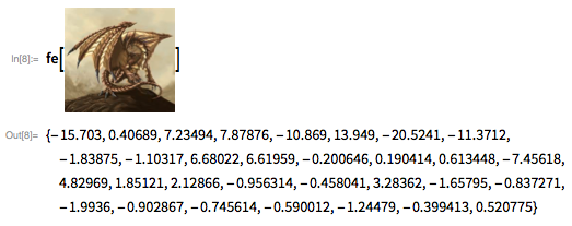
We can then extract features from the first image:

In this case, a vector of length 31 is extracted (a huge data reduction from the 255,600 pixel values in the original image). This extraction is again done in two steps: first, a built-in extractor, specializing in images, is used to extract about 1,000 features from each image. Then a dimensionality reducer is trained from the resulting data to reduce the number of features down to 31. The resulting vectors are much more useful than raw pixel values. For example, let’s say that one wants to find images in the original dataset that are similar to the following query images:

We can try to solve this task using Nearest directly on images:

Some search results make sense, but many seem odd. This is because, by default, Nearest uses a simple distance function based on pixel values, and this is probably why the white unicorn is matched with a white dragon. Now let’s use Nearest again, but in the space of features defined by the extractor function:

This time, the retrieved images seem semantically close to the queries, while their colors can differ a lot. This is a sign that the extractor captures semantic features, and an example of how we can use FeatureExtraction to create useful distances. Another experiment we can do is to further reduce the dimension of the vectors in order to visualize the dataset on a plot:

As you can see, the examples are somewhat semantically grouped (most dragons in the lower right corner, most griffins in the upper right, etc.), which is another sign that semantic features are encoded in these vectors. In a sense, the extractor “understands” the data, and in a sense this is what FeatureExtraction is trying to do.

In the preceding, the “understanding” is mostly due to the first step of the feature extraction process—that is, the use of a built-in feature extractor. This extractor is a byproduct of our effort to develop ImageIdentify. In a nutshell, we took the network trained for ImageIdentify and removed its last layers. The resulting network transforms images into feature vectors encoding high-level concepts. Thanks to the large and diverse dataset (about 10 million images and 10,000 classes) used to train the network, this simple strategy gives a pretty good extractor even for objects that were not in the dataset (such as griffins, centaurs and unicorns). Having such a feature extractor for images is a game-changer in computer vision. For example, if one were to label the above dataset with the classes “unicorn,” “griffin,” etc. and use Classify on the resulting data (as shown here), one would obtain a classifier that correctly classifies about 90% of new images! This is pretty high considering that only eight images per class have been seen during the training. This is not yet a “one-shot learning,” as humans can perform on such tasks, but we are getting there… This result would have been unthinkable in the first versions of Classify, which did not use such an extractor. In a way, this extractor is the visual system of the Wolfram Language. There is still progress to be made, though. For example, this extractor can be greatly enhanced. One of our jobs now is to train other feature extractors in order to boost machine learning performance for all classic data types, such as image, text and sound. I often think of these extractors, and trained models in general, as a new form of built-in knowledge added to the Wolfram Language (along with algorithms and data).

The second step of the reduction, called dimensionality reduction (also sometimes “embedding learning” or “manifold learning”), is the “learned” part of the feature extraction. In the example above, it is probably not the most important step to obtain a useful representation, but it can play a key role for other data types, or when the number of examples is higher (since there is more to learn from). Dimensionality reduction stems from the fact that, in a typical dataset, examples are not uniformly distributed in their original space. Instead, most examples are lying near a lower-dimensional structure (think of it as a manifold). The data examples can in principle be projected on this structure and thus represented with fewer variables than in their original space. Here is an illustration of a two-dimensional dataset reduced to a one-dimensional dataset:

The original data (blue points) is projected onto a uni-dimensional manifold (multi-color curve) that is learned using an autoencoder (see here for more details). The colors indicate the value of the (unique) variable in the reduced space. This procedure can also be applied to more complex datasets, and given enough data and a powerful-enough model, much of the structure of the data can be learned. The representation obtained can then be very useful for downstream tasks, because the data has been “disentangled” (or more loosely again, “understood”). For example, you could train a feature extractor for images that is just as good as our built-in extractor using only dimensionality reduction (this would require a lot of data and computational power, though). Also, reducing the dimension in such a way has other advantages: the resulting dataset is smaller in memory, and the computation time needed to run a downstream application is reduced. This is why we apply this procedure to extract features even in the image case.

We talked about extracting numeric vectors from data in an automatic way, which is the main application of FeatureExtraction, but there is another application: the possibility of creating customized data processing pipelines. Indeed, the second argument can be used to specify named extraction methods, and more generally, named processing methods. For example, let’s train a simple pipeline that imputes missing data and then standardizes it:

We can now use it on new data:

Another classic pipeline, often used in text search systems, consists of segmenting text documents into their words, constructing tf–idf (term frequency–inverse document frequency) vectors and then reducing the dimension of the vectors. Let’s train this pipeline using the sentences of Alice in Wonderland as documents:

The resulting extractor converts each sentence into a numerical vector of size 144 (and a simple distance function in that space could be used to create a search system).

One important thing to mention is that this pipeline creation functionality is not as low-level as one might think; it is a bit automatized. For example, methods such as tf–idf can be applied to more than one data type (in this case, it will work on nominal sequences, but also directly on text). More importantly, methods are only applied to data types they can deal with. For example, in this case the standardization is only performed on the numerical variable (and not on the nominal one):

These properties make it quite handy to define processing pipelines when many data types are present (which is why Classify, Predict, etc. use a similar functionality to perform their automatic processing), and we hope that this will allow users to create custom pipelines in a simple and natural way.

FeatureExtraction is a versatile function. It offers the possibility to control processing pipelines for various machine learning tasks, but also unlocks two new applications: dataset visualization and metric learning for search systems. FeatureExtraction will certainly become a central function in our machine learning ecosystem, but there is still much to do. For example, we are now thinking of generalizing its concept to supervised settings, and there are many interesting cases here: data examples could be labeled by classes or numeric values, or maybe ranking relations between examples (such as “A is closer to B than C”) could be provided instead. Also, FeatureExtraction is another important step in the domain of unsupervised learning, and like ClusterClassify, it enables us to learn something useful about the data—but sometimes we need more than just clusters or an embedding. For example, in order to randomly generate new data examples, predict any variable in the dataset or detect outliers, we need something better: the full probability distribution of the data. It is still a long shot, but we are working to achieve this milestone, probably through a function called LearnDistribution.

To download this post as a CDF, click here. New to CDF? Get your copy for free with this one-time download.