Waiting in line is a common, though not always pleasant, experience for us all. We wait patiently to be served by the next free teller at a bank, clear the security check at an airport, or be answered by technical support when we call a phone service provider. At a more abstract level, these waiting lines, or queues, are also encountered in computer and communication systems. For example, every email you send is broken up into a series of packets. Each packet is then sent off to its destination by the best available route to avoid the queues formed by other packets in the network. Hence, queues play an important role in our lives, and it seems worthwhile to spend some time understanding their dynamics, with a view to answering questions such as, “How many tellers does your bank need to provide good customer service?” or “How can you speed up the security check?” or “On average, how long will you have to wait for technical support?” My purpose in writing this post is to give a gentle introduction to queueing theory, which attempts to answer such questions, using new functions that are available in Mathematica 9.

Queueing theory has its origins in the research of the Danish mathematician A. K. Erlang (1878–1929). While working for the Copenhagen Telephone Company, Erlang was interested in determining how many circuits and switchboard operators were needed to provide an acceptable telephone service. This investigation resulted in his seminal paper “The Theory of Probabilities and Telephone Conversations,” which was published in 1909. Erlang proved that the arrivals for such queues can be modeled as a Poisson process, which immediately made the problem mathematically tractable. Another major advance was made by the American engineer and computer scientist Leonard Kleinrock (1934–), who used queueing theory to develop the mathematical framework for packet switching networks, the basic technology behind the internet. Queueing theory has continued to be an active area of research and finds applications in diverse fields such as traffic engineering and hospital emergency room management.

In 1953, the English mathematician and statistician D. G. Kendall suggested a convenient notation for the mathematical description of queues. According to Kendall’s notation, a queue with arrival time distribution A, service time distribution B, and c servers is called an A/B/c queue. Thus, a single-server queue in which the arrival and service times both follow an exponential distribution is called an M/M/1 queue (the M denotes the “memory-less” property of the exponential distribution). In Mathematica 9, an M/M/1 queue with an arrival rate of 3 customers per minute and a service rate of 5 customers per minute can be defined using the QueueingProcess function as follows.

Let’s simulate this queue for 10 minutes using RandomFunction.

Here is a plot of the simulation that shows the number of customers in the system at any given time during the first 10 minutes.

Notice that the number of waiting customers in the above example does not grow very much, due to the fact that the service rate exceeds the arrival rate. We now consider an M/M/1 queue in which the arrival rate (5 customers per minute) is greater than the service rate (2 customers per minute). As the plot below shows, the number of waiting customers grows without bounds when the queue is simulated over a long period of time.

The above examples would lead us to guess that if the arrival rate for an M/M/1 queue is λ and the service rate is μ, then a steady state is reached provided that λ is less than μ. This is indeed the case, and, under the condition λ < μ, it is possible to compute certain key performance measures for the queue. Two important performance measures are the average number of customers in the system (L) and the average time spent by a customer in the system (W). There is a remarkable relationship between L and W that was established by the American operations research scientist John Little in 1961. Little’s law is widely applied in queueing theory and states that L = λ W. This relationship can be verified using QueueProperties as follows.

Queueing theory provides the basis for efficient management of modern call centers. Since a majority of call center operating costs are related to personnel, getting the right number of staff in place is critical in terms of both service and cost. Imagine then that a call center receives 130 calls per hour and that its team of 20 operators takes an average of 6.8 minutes to answer a call. The probability that a caller will have to wait because all the operators are busy (i.e. that he or she will receive the familiar “Your call is very important to us…” message) is given by the Erlang C formula. For this example, the ErlangC function in Mathematica 9 informs us that the delay probability for a caller is approximately 0.14; that is, around 86% of callers will get an immediate response when they contact the center.

As shown below, the Erlang C formula has a representation of the incomplete Gamma function, and hence it can be computed efficiently to any desired level of precision in Mathematica.

Finally, the call center manager will usually be interested in knowing the number of telephone lines required to ensure an acceptable level of delay probability. This can be accomplished rather easily by building a calculator using the dynamic capabilities of Mathematica, as shown below.

The queues that we encounter in real life are often part of a chain or network of queues. For example, passengers arriving at a major airport will have to make their way through a complicated network of queues for checking in luggage, security scans, and boarding flights to different destinations. Thus, the study of queueing networks, which we shall now discuss, is of great importance in applications.

The two most basic types of queueing networks are open networks and closed networks. In an open network, customers may enter or leave the system at one or more nodes. The study of open networks was revolutionized by J. R. Jackson when he proved that, under reasonable conditions, such a network could be regarded as a “product” of individual M/M/c queues. This dramatic simplification allows one to reuse the formulas that have been derived for single queues. A similar analysis applies to closed queueing networks that have the additional property that the number of customers in the system is fixed, since there are no arrivals or departures at any node. A good example of a closed network might be to consider a university at which a large but fixed number of Mathematica licenses are distributed by the central MathLM server and circulate among the students and faculty. The performance analysis of closed queueing networks relies on techniques developed by W. G. Gordon, G. F. Newell, J. P. Buzen (who famously taught Bill Gates a course on operating systems at Harvard), and others.

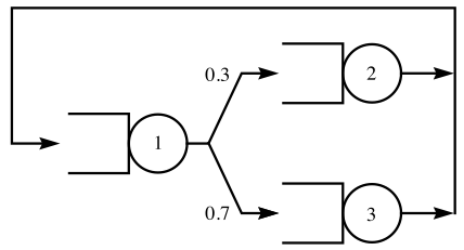
As an example of a queueing network, let’s consider a situation in which 10 requests circulate inside a three-node central server system. The central server (node 1) sends requests with probabilities 0.3 and 0.7 to the remaining two nodes. The service rates at the three nodes are 1, 0.5, and 1.25, respectively. The problem is to find the bottleneck device in this closed network of servers.

The central server network can be modeled using the QueueingNetworkProcess function in Mathematica 9, as shown below. The first argument of QueueingNetworkProcess is the zero vector, since the network is closed and hence there are no arrivals from outside at any node. The second argument is the matrix of routing probabilities, for example, 0.3 is the probability that a request will travel from node 1 to node 2 after leaving node 1. The third argument is the vector of service rates as given in the statement of the problem. The fourth argument indicates that there is only one server at each node. Finally, the fifth argument specifies the total number of requests, 10, that circulate in this closed network.

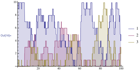
As seen from the simulation below, the first node appears to be the bottleneck device, since the traffic is concentrated at this node for a major portion of the time.

The bottleneck can be cleared by allotting more resources to increase the service rate at the first node. The improvement can be visualized using the Manipulate function after allowing the service rate to be a symbolic parameter μ as shown below.

Queueing theory is a perfect example of applied mathematics for the computer and information age that we live in. Its simple principles, elegant theorems, and broad applicability will ensure that it remains an important field of study in the years to come. I hope that this brief introduction will motivate you to delve deeper into this fascinating subject using the new functions for queueing processes in Mathematica 9. A video based on my recent talk at the Wolfram Technology Conference is also available. Any comments on the new functionality are, of course, very welcome.

Credit: The image below the title of the blog post is a reproduction of the painting Noah’s Ark by Edward Hicks (1780–1849).

Download this post as a Computable Document Format (CDF) file.