What is the cost of extending a warranty for a car? I’d be interested to know, since my car broke down just past the 100,000 mile marker on a road trip through America. With Mathematica 9 comes complete functionality for reliability analysis that can help us analyze systems like cars. I thought it might be worthwhile to take Mathematica for a spin and look at how some technical systems can be modeled and analyzed.

As an example, take the engine of my Mitsubishi Diamante. In order to work, the Mitsubishi V6 engine needs spark plugs, gasoline direct injection, and a timing belt. This can be modeled with ReliabilityDistribution:

The function ReliabilityDistribution takes two arguments: a Boolean expression describing the layout of the system and probability distributions describing the individual components’ lifetimes. I’m using ∧ for the And operator in the above input; Mathematica can handle “And,” ” ∧,” and “&&” for the And operator and similarly, “∨,” “||,” and “Or” for the Or operator.

The lifetime distributions can be the typical distributions used in the field, such as Weibull, exponential, gamma, log-normal, Erlang, Birnbaum–Saunders, and many more. Here I’m using both the Weibull and the exponential distributions and assuming that the average failure of the gasoline direct injection system occurs at around 220,000 miles, 75,000 miles for the timing belt, and 145,000 miles for the spark plugs.

Now I can easily query the system for various properties such as the mean time to failure (MTTF), which is about 53,000 miles:

Or plot the survival function, sometimes called the reliability function.

In short, all of the probability and statistics functions work with ReliabilityDistribution.

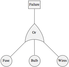
Another subsystem of my car that I recently had to familiarize myself with is the rear lighting system. This system will fail if the light bulb burns out, the fuse blows, or the electrical wires are broken. This failure-oriented approach can be modeled with a FailureDistribution.

Here I’m using three different failure rates for the light bulbs, the fuse, and the wires. The coefficients in front of the parameter λ reflect my experience that the bulbs blow more often than the fuses, which in turn are less prone to faults than the wires. I’ll keep λ, the failure rate in months, symbolic to start with and use numeric values when needed.

Just as with the ReliabilityDistribution, I can calculate properties for this system. Symbolic computations are of course directly supported. Here is the probability that the system fails before time t==1/2.

To create more elaborate models, I usually structure my models into hierarchies. So if I want to model both the front and the rear lights, I can do that with a hierarchical system by combining two ReliabilityDistributions into one, separating them by a Boolean expression—in this case an And operation.

By setting λ to 100 months, I can plot the survival function for the system:

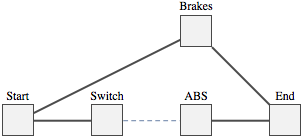
My car is also equipped with a traction control system and anti-lock braking system (ABS). If the ABS fails, the car reverts to using the regular braking system. This fallback mechanism can be modeled with a StandbyDistribution. For the ABS to work, both the electronic control unit (ECU) and the two wheel sensors need to work.

I start with creating a reliability distribution for the ABS and with two separate symbolic failure rates λ₁ and λ₂.

Then I can create a distribution for how the complete brake system works.

OK, so say I have the components, their lifetimes, and their configuration. Now how do I find out which components to improve? This question is exactly what the so-called importance measures are for. As an example, I’ll look at my anti-lock braking system and figure out which components to improve.

Improvement importance (sometimes also called improvement potential) describes how much the survival function of a component would increase if it were replaced by a perfect component, making it easy to see which components to increase the reliability of. If you have economic data, it’s also easy to make economically sound decisions. The improvement importance is a relative measure, so for a figure to make sense, it has to be put in context with the other components in the system.

In this case, it’s not surprising to see that the left- and right-wheel sensors show the same importance (they have the same structural importance and the same lifetime distribution). By adding some numbers to the failure rates, assuming the sensor breaks on average after 10,000 hours and the ECU after 25,000 hours, I can plot the system.

Given these numbers, one should first improve the sensors before improving the ECU, since they show higher improvement potential throughout. This agrees with my and other Diamante owners’ experience, when my sensors have failed while the ECU is fine. The sensors are easy to replace, but (relatively) expensive.

Finally, let’s return to my opening question and the pricing of warranty policies. What should an extension of the warranty from 100,000 miles to 150,000 miles cost?

With a mean cost of repair at $1,000, it would turn out to be around $96:

If you are interested in learning about the capabilities of the reliability functionality in Mathematica, you can watch this presentation I did at last year’s Wolfram Technology Conference.

Or go right to the documentation.

Download this post as a Computable Document Format (CDF) file.