Mathematica and the Fundamental Theorem of Calculus
Most calculus students might think that if one could compute indefinite integrals, it would always be easy to compute definite ones. After all, they might think, the fundamental theorem of calculus says that one just has to subtract the values of the indefinite integral at the end points to get the definite integral.
So how come inside Mathematica there are thousands of pages of code devoted to working out definite integrals—beyond just subtracting indefinite ones?
The answer, as is often the case, is that in the real world of mathematical computation, things are more complicated than one learns in basic mathematics courses. And to get the correct answer one needs to be considerably more sophisticated.
In a simple case, subtracting indefinite integrals works just fine.
Consider computing the area under a sine curve, which equals ![]()
![In[1]= Show[<br> Plot[Sin[x], {x, 0, 2Pi}, Ticks -> {Range[0, 8] Pi/4, Automatic}, PlotLabel->Sin[x]], RegionPlot[Sin[x]>y&&y>0, {x, 0, Pi}, {y, 0, 1}, ColorFunction -> (None&), MeshFunctions -> {#1 - #2&}, Mesh -> 20, Frame -> False, Axes -> True, BoundaryStyle -> None], Plot[Sin[x], {x, 0, 2Pi}, Ticks -> {Range[0, 8]Pi/4, Automatic}], ImageSize->Small]](https://content.wolfram.com/sites/39/2021/01/duplicate_pavlyk_2.gif "In[1]= Show[<br> Plot[Sin[x], {x, 0, 2Pi}, Ticks -> {Range[0, 8] Pi/4, Automatic}, PlotLabel->Sin[x]], RegionPlot[Sin[x]>y&&y>0, {x, 0, Pi}, {y, 0, 1}, ColorFunction -> (None&), MeshFunctions -> {#1 - #2&}, Mesh -> 20, Frame -> False, Axes -> True, BoundaryStyle -> None], Plot[Sin[x], {x, 0, 2Pi}, Ticks -> {Range[0, 8]Pi/4, Automatic}], ImageSize->Small]")
We work out the indefinite integral:
![In[2]= f[x_] = \[Integral]Sin[x] \[DifferentialD]x](https://content.wolfram.com/sites/39/2021/01/duplicate_pavlyk_3.gif "In[2]= f[x_] = \[Integral]Sin[x] \[DifferentialD]x")
Then we can just subtract its value at each end point, and correctly find a definite integral such as ![]()
![]()
But consider a more complicated case:
![In[4]= f[x_] = \[Integral]1/(5 + 4 Sin[x]) \[DifferentialD]x // Simplify](https://content.wolfram.com/sites/39/2021/01/duplicate_pavlyk_6.gif "In[4]= f[x_] = \[Integral]1/(5 + 4 Sin[x]) \[DifferentialD]x // Simplify")
We can verify that this indefinite integral at least formally differentiates correctly:
![In[5]= D[f[x], x] // Simplify](https://content.wolfram.com/sites/39/2021/01/duplicate_pavlyk_7.gif "In[5]= D[f[x], x] // Simplify")
Now let’s compute the definite integral ![]() by subtracting values of our indefinite one:
by subtracting values of our indefinite one:
![]()
But this cannot be correct. After all, if we plot the integrand, we can see that it is positive throughout the range 0 to 2π:
![In[7]= Plot[1/(5+4Sin[x]), {x, 0, 2Pi}, ImageSize -> Small, Filling -> Axis, AxesOrigin -> {0, 0}, Ticks -> {{0, Pi/2, Pi, 3Pi/2, 2Pi}, Automatic}, Epilog -> Inset[Framed[Style[TraditionalForm[HoldForm[(5 + 4Sin[x])^ -1]], Larger, Black], Background -> GrayLevel[0.95]], {(11 \[Pi])/16, 0.8}]]](https://content.wolfram.com/sites/39/2021/01/duplicate_pavlyk_10.gif "In[7]= Plot[1/(5 + 4Sin[x]), {x, 0, 2Pi}, ImageSize -> Small, Filling -> Axis, AxesOrigin -> {0, 0}, Ticks -> {{0, Pi/2, Pi, 3Pi/2, 2Pi}, Automatic}, Epilog -> Inset[Framed[Style[TraditionalForm[HoldForm[(5 + 4Sin[x])^ -1]], Larger, Black], Background -> GrayLevel[0.95]], {(11 \[Pi])/16, 0.8}]]")
Mathematica’s built-in definite integration of course gives exactly the correct answer:
![In[8]= \!\(<br> \*SubsuperscriptBox[\(\[Integral]\), \(0\), \(2\ \[Pi]\)]\(<br> FractionBox[\(1\), \(5 + 4\ Sin[x]\)] \[DifferentialD]x\)\)](https://content.wolfram.com/sites/39/2021/01/duplicate_pavlyk_11.gif "In[8]= \!\(<br> \*SubsuperscriptBox[\(\[Integral]\), \(0\), \(2\ \[Pi]\)]\(<br> FractionBox[\(1\), \(5 + 4\ Sin[x]\)] \[DifferentialD]x\)\)")
So what went wrong with subtracting the end points? The issue is that the fundamental theorem of calculus isn’t directly applicable here. Because, when you state it fully, the theorem requires that the antiderivative that is going to be subtracted be continuous throughout the interval.
But the antiderivative we have here looks like this:
![In[9]= Labeled[Plot[f[x], {x, 0, 2Pi}, Exclusions -> Pi, ExclusionsStyle -> {Dashed}, ImageSize -> Small, AxesOrigin -> {0, - 1}, Ticks -> {{0, Pi/2, Pi, 3Pi/2, 2Pi}, Automatic}], TraditionalForm[HoldForm@f[x]]]](https://content.wolfram.com/sites/39/2021/01/duplicate_pavlyk_12.gif "In[9]= Labeled[Plot[f[x], {x, 0, 2Pi}, Exclusions -> Pi, ExclusionsStyle -> {Dashed}, ImageSize -> Small, AxesOrigin -> {0, - 1}, Ticks -> {{0, Pi/2, Pi, 3Pi/2, 2Pi}, Automatic}], TraditionalForm[HoldForm@f[x]]]")
It has a discontinuity right in the middle of the interval.
So how does Mathematica get its answer? It has to be more careful. Sometimes it works by detecting discontinuities in the antiderivative, and then breaking up the integration region into parts, and carefully taking directional limits at the discontinuity points:
![In[10]= (f[2 \[Pi]]-Limit[f[\[Pi] + \[Epsilon]],\[Epsilon] -> 0]) + (Limit[f[\[Pi] - \[Epsilon]], \[Epsilon] -> 0] - f[0])](https://content.wolfram.com/sites/39/2021/01/duplicate_pavlyk_13.gif "In[10]= (f[2 \[Pi]]-Limit[f[\[Pi] + \[Epsilon]],\[Epsilon] -> 0]) + (Limit[f[\[Pi] - \[Epsilon]], \[Epsilon] -> 0] - f[0])")
Another thing it can do is to make use of ambiguity in the antiderivative. Every calculus student knows that antiderivatives can contain an arbitrary additive constant. But in fact, there’s more arbitrariness than that: one can add different constants on different parts of the interval.
Often it’s not obvious from the algebraic form that one has added a piecewise constant like this. For example, consider:
![]()
Differentiating this shows that it is indeed an antiderivative of the same function as above.
![In[12]= D[Subscript[f, c][x], x] // Simplify](https://content.wolfram.com/sites/39/2021/01/duplicate_pavlyk_15.gif "In[12]= D[Subscript[f, c][x], x] // Simplify")
It doesn’t happen to be the antiderivative that Mathematica generates by default. But it is a perfectly valid one. And it turns out to be continuous over the region of integration:
![In[13]= Labeled[Plot[Subscript[f, c][x], {x, 0, 2Pi}, ImageSize -> Small, AxesOrigin -> {0, 0}, Ticks -> {{0, Pi/2, Pi, 3Pi/2, 2Pi}, Automatic}], TraditionalForm[HoldForm@Subscript[f,c][x]]]](https://content.wolfram.com/sites/39/2021/01/duplicate_pavlyk_16.gif "In[13]= Labeled[Plot[Subscript[f, c][x], {x, 0, 2Pi}, ImageSize -> Small, AxesOrigin -> {0, 0}, Ticks -> {{0, Pi/2, Pi, 3Pi/2, 2Pi}, Automatic}], TraditionalForm[HoldForm@Subscript[f,c][x]]]")
So if one uses it, one can now directly apply the fundamental theorem of calculus and get the correct result:
![In[14]= Subscript[f, c][2 Pi] - Subscript[f, c][0] // Expand](https://content.wolfram.com/sites/39/2021/01/duplicate_pavlyk_17.gif "In[14]= Subscript[f, c][2 Pi] - Subscript[f, c][0] // Expand")
Even though their algebraic forms look different, one can verify that the antiderivatives differ by a piecewise constant:
![In[15]= Labeled[Plot[Subscript[f,c][x] - f[x], {x, 0, 2Pi}, ImageSize -> Small, AxesOrigin -> {0, Pi/3}, Ticks -> {{0, Pi/2, Pi, 3Pi/2, 2Pi}, {-Pi/6, 0, Pi/6, Pi/3, Pi/2, 2Pi/3}}], TraditionalForm[HoldForm[Subscript[f, c][x] - f[x]]]]](https://content.wolfram.com/sites/39/2021/01/duplicate_pavlyk_18.gif "In[15]= Labeled[Plot[Subscript[f,c][x] - f[x], {x, 0, 2Pi}, ImageSize -> Small, AxesOrigin -> {0, Pi/3}, Ticks -> {{0, Pi/2, Pi, 3Pi/2, 2Pi}, {-Pi/6, 0, Pi/6, Pi/3, Pi/2, 2Pi/3}}], TraditionalForm[HoldForm[Subscript[f, c][x] - f[x]]]]")
So how come Mathematica doesn’t always generate the “better” antiderivative, so that the fundamental theorem of calculus applies directly?
The problem is that there’s actually no way to produce an antiderivative that has this property for all definite integrals one might want to compute. Here’s the formal situation.
The fundamental theorem of calculus states that an antiderivative continuous along a chosen path always exists. It is defined as ![]() , where the integration is performed along the path. Its existence is of theoretical importance—though in practice
, where the integration is performed along the path. Its existence is of theoretical importance—though in practice ![]() cannot always be expressed in terms of any predetermined set of elementary and special functions.
cannot always be expressed in terms of any predetermined set of elementary and special functions.
Moreover, if a meromorphic integrand ![]() has simple poles in the complex plane, it is impossible to choose an antiderivative
has simple poles in the complex plane, it is impossible to choose an antiderivative ![]() continuous along every imaginable path in the complex plane—because of branch cuts in
continuous along every imaginable path in the complex plane—because of branch cuts in ![]() .
.
Our integrand ![]() has simple poles at
has simple poles at ![]() :
:
![In[16]= {Series[1/(5 + 4 Sin[z]), {z, - (Pi/2) + I Log[2], 0}],<br> Series[1/(5 + 4 Sin[z]), {z, - (Pi/2) - I Log[2], 0}]}](https://content.wolfram.com/sites/39/2021/01/duplicate_pavlyk_26.gif "In[16]= {Series[1/(5 + 4 Sin[z]), {z, - (Pi/2) + I Log[2], 0}], Series[1/(5 + 4 Sin[z]), {z, - (Pi/2) - I Log[2], 0}]}")
But now consider how our two antiderivatives behave in the complex plane. Here are the real parts of these functions:
![In[17]= {Labeled[Show[<br> Plot3D[Re[Subscript[f, c][x+I y]], {x, -Pi, 3Pi}, {y, -2, 2}, ImageSize -> 300, ViewPoint -> {-1, 2, 3/2}, AxesLabel -> {x, y, HoldForm@Re[Subscript[f, c][x+I y]]}],<br> ParametricPlot3D[{x, 3/2, Re[Subscript[f, c][x + 3/2I]]}, {x, 0, 2Pi}, PlotStyle -> {Black, Tube[0.05]}]<br> ], TraditionalForm[HoldForm@Subscript[f, c][x]]], Spacer[15], Labeled[Show[<br> Plot3D[Re[f[x + Iy]], {x, - Pi, 3Pi}, {y, -2, 2}, ImageSize -> 300, ViewPoint -> {-1, 2, 3/2}, AxesLabel -> {x, y, HoldForm@Re[f[x + Iy]]}], ParametricPlot3D[{x, 3/2, Re[f[x + 3/2I]]}, {x, 0, 2Pi}, PlotStyle -> {Black, Tube[0.05]}]], TraditionalForm[HoldForm@f[x]]]}//Reverse//Row](https://content.wolfram.com/sites/39/2021/01/duplicate_pavlyk_27.gif "In[17]= {Labeled[Show[<br> Plot3D[Re[Subscript[f, c][x+I y]], {x, -Pi, 3Pi}, {y, -2, 2}, ImageSize -> 300, ViewPoint -> {-1, 2, 3/2}, AxesLabel -> {x, y, HoldForm@Re[Subscript[f, c][x + I y]]}],<br> ParametricPlot3D[{x, 3/2, Re[Subscript[f, c][x + 3/2I]]}, {x, 0, 2Pi}, PlotStyle -> {Black, Tube[0.05]}]<br> ], TraditionalForm[HoldForm@Subscript[f, c][x]]], Spacer[15], Labeled[Show[<br> Plot3D[Re[f[x + I y]], {x, - Pi, 3Pi}, {y, -2, 2}, ImageSize -> 300, ViewPoint -> {-1, 2, 3/2}, AxesLabel -> {x, y, HoldForm@Re[f[x + I y]]}], ParametricPlot3D[{x, 3/2, Re[f[x + 3/2I]]}, {x, 0, 2Pi}, PlotStyle -> {Black, Tube[0.05]}]], TraditionalForm[HoldForm@f[x]]]}//Reverse//Row")
Looking on the real axis, ![]() is not continuous, so the fundamental theorem cannot directly be applied. But
is not continuous, so the fundamental theorem cannot directly be applied. But ![]() is continuous, so the fundamental theorem will work.
is continuous, so the fundamental theorem will work.
However, look now at the line from ![]() , indicated in the picture by a black line. Along this line,
, indicated in the picture by a black line. Along this line, ![]() is continuous, so the fundamental theorem will work fine for it. But now
is continuous, so the fundamental theorem will work fine for it. But now ![]() is not continuous, so the fundamental theorem will not work:
is not continuous, so the fundamental theorem will not work:
![In[18]= With[{z0 = 3/2I, z1 = 2Pi + 3/2I}, {\!\(<br> \*SubsuperscriptBox[\(\[Integral]\), \(z0\), \(z1\)]\(<br> FractionBox[\(1\), \(5 + 4\ Sin[x]\)] \[DifferentialD]x\)\), Subscript[f, c][z1] - Subscript[f, c][z0], f[z1] - f[z0]}//Simplify]](https://content.wolfram.com/sites/39/2021/01/duplicate_pavlyk_33.gif "In[18]= With[{z0 = 3/2I, z1 = 2Pi + 3/2I}, {\!\(<br> \*SubsuperscriptBox[\(\[Integral]\), \(z0\), \(z1\)]\(<br> FractionBox[\(1\), \(5 + 4\ Sin[x]\)] \[DifferentialD]x\)\), Subscript[f, c][z1] - Subscript[f, c][z0], f[z1] - f[z0]}//Simplify]")
And indeed one can show that there is no single choice of antiderivative for which the fundamental theorem will always work.
So Mathematica has to go to more effort to get the correct answer for the definite integral.
This may seem subtle—but actually it is just the tip of the iceberg of the issues that crop up in doing definite integration correctly in Mathematica—and in mathematics. It’s the job of our group at Wolfram Research to understand all these issues and figure out good algorithms for handling them. It’s a fascinating exercise not only in algorithm development but also in mathematics itself.